CS6015: Linear Algebra and Random Processes

Lecture 28: Probability Space, Axioms of Probability, Designing Probability Functions

Probability Theory

Basics

Laws

Random Var.

Applications

Processes

Counting

Set Theory

Axioms

Union rule

Multiplication Rule

Total Probability Theorem

Bayes' Theorem

Independence

\mathbb{P}: \mathcal{F} \rightarrow [0,1]

X: \mathcal{\Omega} \rightarrow \mathbb{R}

PMF, PDF, CDF

Expectation, Var., Moments

Distributions (~10)

Bayes' Theorem

Independence

Sampling from a distribution

Designing arbitrary probability functions

Estimating Parameters

X_1, X_2, \dots, X_t,\dots

Simple Random Walk

Bernoulli Process

Poisson Process

Markov Process

.... .... ....

Limit Theorems

Markov inequality

Chebychev inequality

Weak Law of large nos.

Central Limit Theorem

The

St

Joint, cond., marginal dist.

(ML)

.... .... ....

Learning Objectives

What is a probability space?

What are the axioms of probability?

What are some simple ways of defining a probability function?

Probability Space

Definitions

$\Omega$: Sample space (all outcomes)

Event: subsets of $\Omega$

Field $\mathcal{F}$: a subcollection of the set of all subsets of $\Omega$ such that

if $A,B \in \mathcal{F}$ then $A\cap B \in \mathcal{F}$ and $A\cup B \in \mathcal{F}$

if $A \in \mathcal{F}$ then $A^\mathsf{c} \in \mathcal{F}$

$\phi\in \mathcal{F}$

(empty set)

Why not simply say all subsets of $\Omega$ ?

(beyond the scope of this course)

Definitions

$\sigma$-field $\mathcal{F}$: A collection of the subsets of $\Omega$ is called a $\sigma$-field if

if $A_1,A_2, \dots \in \mathcal{F}$ then $\cup_{i=1}^{\infty} A_i \in \mathcal{F}$

if $A \in \mathcal{F}$ then $A^\mathsf{c} \in \mathcal{F}$

$\phi\in \mathcal{F}$

(empty set)

if $A_1,A_2, \dots \in \mathcal{F}$ then $\cap_{i=1}^{\infty} A_i \in \mathcal{F}$

closed under countable unions & intersections

The power set of $\Omega$ which contains ALL subsets of $\Omega$ is obviously a $\sigma$-field

Definitions

a probability measure $\mathbb{P}$ on $\Omega, \mathcal{F}$ is a function $\mathbb{P}: \mathcal{F} \rightarrow [0,1] $ satisfying the axioms of probability

The triple $(\Omega, \mathcal{F}, \mathbb{P})$ where $\mathcal{F}$ is a $\sigma$-field, is called a probability space

(we will soon see what these axioms are)

Recap

Experiments

Sample Space

Events

What is the chance of an event?

Goal: Assign a number to each event such that this number reflects the chance of the experiment resulting in that event

($\sigma$-field $\mathcal{F}$)

The probability function

What are the conditions that such a probability function must satisfy?

(Axioms of Probability)

P(A) = ?

Event

Probability function

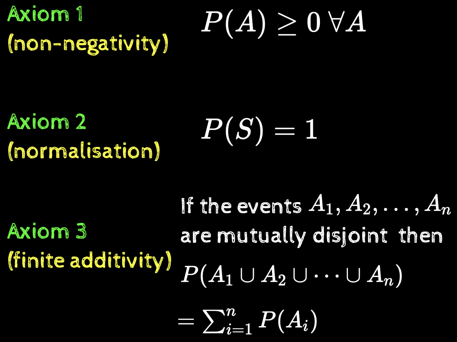
The axioms of probability

P(A) \geq 0~\forall A

Axiom 1 (non-negativity)

P(\Omega) = 1

Axiom 2 (normalisation)

Axiom 3 (finite additivity)

If the events are mutually disjoint then

A_1, A_2, \dots, A_n

= \sum_{i=1}^n P(A_i)

P(A_1\cup A_2 \cup \dots \cup A_n)

The axioms of probability

Axiom 3 (finite additivity)

= \sum_{i=1}^n P(A_i)

P(A_1\cup A_2 \cup \dots \cup A_n)

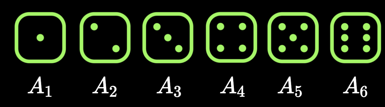
Smallest possible event = one outcome

Compute probabilities of larger events from smaller events

A_1

A_2

A_3

A_4

A_5

A_6

The axioms of probability

Given

P(A_1),P(A_2),P(A_3),P(A_4),P(A_5),P(A_6)

: the event that the outcome is an odd no.

: the event that the outcome is

P(B) = P(A_1)+P(A_3)+P(A_5)

\geq 5

P(C) = P(A_5)+P(A_6)

: the event that the outcome is a mult. of 3

P(D) = P(A_3)+P(A_6)

we can compute other probabilities

The probability of an event can be computed as the sum of the probabilities of the disjoint outcomes contained in the event

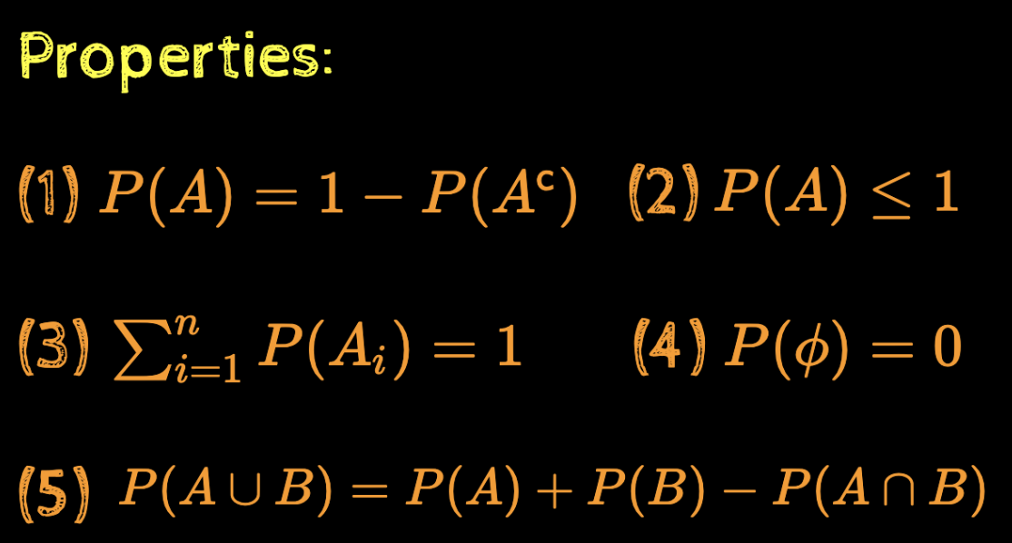
Some properties of probability

Property 1:

P(A) = 1 - P(A^\mathsf{c})

A \cup A^\mathsf{c} = \Omega

1 = P(\Omega) = P(A \cup A^\mathsf{c}) = P(A) + P(A^\mathsf{c})

\therefore P(A) = 1 - P(A^\mathsf{c})

Property 2:

P(A) \leq 1

P(A) = 1 - P(A^\mathsf{c})

Some properties of probability

Property 3:

P(A \cup B) = P(A) + P(B) - P(A \cap B)

A^\mathsf{c}

P(A \cup B) = P(A \cup (B \cap A^\mathsf{c}))

= P(A) + P(B \cap A^\mathsf{c})

P(B) = P((B \cap A^\mathsf{c}) \cup (B \cap A))

= P(B\cap A^\mathsf{c}) + P(B\cap A)

\therefore P(B\cap A^\mathsf{c}) = P(B) - P(B\cap A)

= P(A) + P(B) - P(B\cap A)

Some properties of probability

Property 4:

\Omega = A_1 \cup A_2 \cup \dots \cup A_n

the sum of the probabilities of all outcomes is equal to 1

P(\Omega) = P(A_1 \cup A_2 \cup \dots \cup A_n) = \sum_{i=1}^n P(A_i)

\therefore \sum_{i=1}^n P(A_i) = 1

\underbrace{~~~~~~~~~~~~~~~~~~~~~~~~~~~~~~~~~~~~~~~~}

\Omega

Property 5:

P(\phi) = 0

\therefore 1 = P(\Omega) = P(\Omega \cup \phi) = P(\Omega) + P(\phi)

\therefore 1 = 1 + P(\phi) \implies P(\phi) = 0

Examples

Outcomes: {0, 1, 2, 3, 4, 5, 6}

A_0, A_1, A_2, A_3, A_4, A_5, A_6

P(A_0)=0.3, P(A_1)=0.45, P(A_2)=0.12, P(A_3)=0.02, \\ P(A_4)=0.07, P(A_5)=0.01, P(A_6)=0.03

What is the prob. of scoring even no. of runs?

X = A_0 \cup A_2 \cup A_4 \cup A_6

P(X) = P(A_0 \cup A_2 \cup A_4 \cup A_6)

= P(A_0) + P(A_2) + P(A_4) + P(A_6)

Examples

Outcomes: {0, 1, 2, 3, 4, 5, 6}

A_0, A_1, A_2, A_3, A_4, A_5, A_6

P(A_0)=0.3, P(A_1)=0.45, P(A_2)=0.12, P(A_3)=0.02, \\ P(A_4)=0.07, P(A_5)=0.01, P(A_6)=0.03

What is the prob. of scoring less than 5 runs?

X = A_0 \cup A_1 \cup A_2 \cup A_3 \cup A_4

P(X) = P(A_0 \cup A_1 \cup A_2 \cup A_3 \cup A_4)

= P(A_0) + P(A_1) + P(A_2) + P(A_3) + P(A_4)

Examples

Outcomes: {0, 1, 2, 3, 4, 5, 6}

A_0, A_1, A_2, A_3, A_4, A_5, A_6

P(A_0)=0.3, P(A_1)=0.45, P(A_2)=0.12, P(A_3)=0.02, \\ P(A_4)=0.07, P(A_5)=0.01, P(A_6)=0.03

The prob. that the runs will be div. by 2 or 3?

X_1 = \{0, 2, 4, 6\} = A_0 \cup A_2 \cup A_4 \cup A_6

X_2 = \{0, 3, 6\} = A_0 \cup A_3 \cup A_6

X_1 \cap X_2 = \{0, 6\} = A_0 \cup A_6

P(X_1) = 0.3 + 0.12 + 0.07 + 0.03 = 0.52

P(X_2) = 0.3 + 0.02 + 0.03 = 0.35

P(X_1 \cap X_2) = 0.3 + 0.03 = 0.33

P(X_1 \cup X_2) = P(X_1) + P(X_2) - P(X_1 \cap X_2)

\therefore P (X_1 \cup X_2) = 0.52 + 0.35 - 0.33 = 0.54

Examples

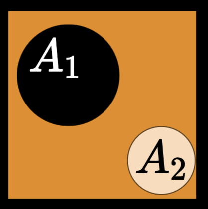
The ball bearings manufactured by a factory have two types of defects. Suppose the probability of having Type 1 defect is 0.01, having Type 2 defect is 0.02 and having both is 0.0005

P(A_1)=0.01, P(A_2)=0.03, P(A_1 \cap A_2) = 0.005

P(A_1 \cup A_2)= P(A_1) + P(A_2) - P(A_1 \cap A_2)

What is the prob. that the bearing will have type 1 or type 2 defect ?

= 0.01 + 0.02 - 0.005 = 0.025

A_2

A_1

Examples

The ball bearings manufactured by a factory have two types of defects. Suppose the probability of having Type 1 defect is 0.01, having Type 2 defect is 0.02 and having both is 0.0005

P(A_1)=0.01, P(A_2)=0.03, P(A_1 \cap A_2) = 0.005

P(A_1 \cup A_2)^\mathsf{c}= 1 - P(A_1 \cup A_2)

What is the prob. that the bearing will have neither type 1 nor type 2 defect ?

= 1 - 0.025 = 0.975

A_2

A_1

Designing Probability Functions

(probability as relative frequency)

Recap

Goal: Assign a number to each event such that this number reflects the chance of the experiment resulting in that event

Required: The probability function must satisfy the axioms of probability

Probability as relative frequency

Karl Pearson tossed a coin 24000 times he observed that the number of heads was 12012

P(H) = \frac{12012}{24000} = 0.5005

We can think of the probability of an event as the fraction of times the event occurs when an experiment is repeated a large number of times

Probability as relative frequency

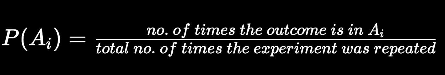
We can think of the probability of an event as the fraction of times the event occurs when an experiment is repeated a large number of times

P(A_i) = \frac{no.~of~times~the~outcome~is~in~A_i}{total~no.~of~times~the~experiment~was~repeated}

But does such a P() satisfy the axioms of probability?

Probability as relative frequency

P(A_i) \geq 0~?

: ratio of two positive numbers

Does P() satisfy the axioms?

P(\Omega)=1~?

P(\Omega) = \frac{no.~of~times~the~outcome~is~in~S}{total~no.~of~times~the~experiment~was~repeated} = 1

\Omega

P(A_1 \cup A_2) = P(A_1)+ P(A_2)~?

P(A_1 \cup A_2) = \frac{k_1 + k_2}{k} = \frac{k_1}{k} + \frac{k_2}{k}

= P(A_1)+ P(A_2)

A_1

A_2

Probability as relative frequency

Does P() satisfy the axioms?

\Omega

P(A_1 \cup A_2) = P(A_1)+ P(A_2)~?

|\Omega| = n \implies 2^n~subsets \implies 2^n~events

A_1, A_2, A_3, \dots, A_n

Suppose are the outcomes

Every event is a union of these outcomes

If the frequencies of are known then the probability of any event can be computed

A_1, A_2, A_3, \dots, A_n

(axioms are about events)

Examples

A dataset contains images of beaches (60000), mountains (25000) and forests (15000)

What is the probability that a randomly picked image would be of a forest?

Experiment: Select an image

Number of trials: 100000

Frequency of the event "forest": 15000

P(forest) = \frac{15000}{100000} = 0.15

Examples

A country tests 20 million randomly selected people and finds that 1 million are infected

What is the probability that a randomly picked person would be infected?

Experiment: Perform a test

Number of trials: 20 million

Frequency of the event "infected": 1 million

P(infected) = \frac{1000000}{20000000} = 0.05

Examples

By May-10-2020, India had tested 1673688 samples of which 67176 were found to be positive. Does this mean the probability that a randomly selected person being infected is 0.04

A subtle point: the sample from which the probabilities were estimated should be drawn from the same population on which we are interested in making inferences

No: testing in India was not random but only for people with flu-like symptoms

Flu

\Omega

Designing Probability Functions

(the case of equally likely outcomes)

Equally likely outcomes

P(H) = P(T) = k

\Omega = H \cup T

P(\Omega) = P(H \cup T)

= P(H) + P(T)

\Omega = \{H, T\}

= 2k

= 1

\therefore P(H) = P(T) = k = \frac{1}{2}

We can now compute the probability of all 4 subsets of

\Omega

\phi, \{H\}, \{T\}, \{H, T\}

Equally likely outcomes

A_i

: event that the out come is i

A_1, A_2, A_3, A_4, A_5, A_6

partition

\Omega

P(A_1) = P(A_2) = P(A_3) = P(A_4) = P(A_5) = P(A_6) = k

P(S) = \sum_{i=1}^6 P(A_i) = 6k = 1

\therefore P(A_i) = \frac{1}{6}

We can now compute the probability of all subsets of

\Omega

\Omega = \{1, 2, 3, 4, 5, 6\}

A_1

A_2

A_3

A_4

A_5

A_6

Equally likely outcomes

We can now compute the probability of all subsets of

\Omega

: outcome is even

\Omega = \{1, 2, 3, 4, 5, 6\}

A_1

A_2

A_3

A_4

A_5

A_6

: outcome is odd

: outcome is divisible by 3

Equally likely outcomes

Can we derive a formula for computing the probability of events of an experiment with n equally likely outcomes?

: any event with k outcomes

(the outcomes are of course disjoint)

P(E) = \sum_{i=1}^{k} \frac{1}{n} = \frac{k}{n}

\frac{1}{n}

P(X) = \frac{number~of~outcomes~in~X}{number~of~outcomes~in~\Omega}

Equally likely outcomes

Are the axioms of probability satisfied?

\frac{1}{n}

P(X) = \frac{number~of~outcomes~in~X}{number~of~outcomes~in~\Omega}

P(A_i) \geq 0~?

: ratio of two positive numbers

P(\Omega)=1~?

P(A_1 \cup A_2) = P(A_1)+ P(A_2)~?

: contains all outcomes

A_1

A_2

P(A_1 \cup A_2) = \frac{k_1 + k_2}{n} = \frac{k_1}{n} + \frac{k_2}{n}

= P(A_1) + P(A_2)

Examples

What is the probability of getting a black card?

\frac{1}{n}

P(B) = \frac{26}{52}

P(X) = \frac{number~of~outcomes~in~X}{number~of~outcomes~in~\Omega}

What is the probability of getting 3 aces?

n = {52 \choose 3} = 22100

P(A) = \frac{4}{22100}

Examples

What is the probability of hitting the red circle at the centre?

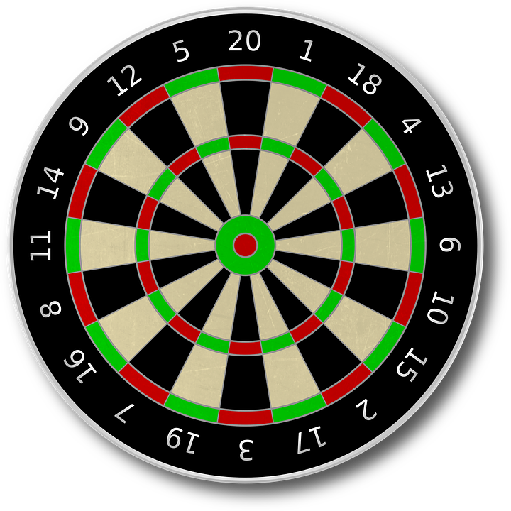
P(C) = \frac{\pi r^2}{\pi R^2} = (\frac{r}{R})^2

: radius of dartboard

: radius of red circle

Countably infinite sample space

Examples

Keep tossing the coin till you get the first head

\Omega = \{1,2,3,\dots\}

... ... ...

Suppose

P(n) = \frac{1}{2^n}

(why? we will see later)

Is this a valid probability distribution?

P(n) \geq 0

P(\Omega) = \sum_{i=1}^{\infty}\frac{1}{2^n} = \frac{1}{2}\sum_{i=0}^{\infty} \frac{1}{2^i} = \frac{1}{2}\cdot\frac{1}{1 - \frac{1}{2}} = 1

Examples

... ... ...

What is the probability that $n$ would be even?

What about the third axiom?

P(outcome~is~even) = P(\{2\} \cup \{4\} \cup \{6\} \cup \dots )

disjoint events

P(outcome~is~even) = P(2) + P(4) + P(6) + \dots

=\frac{1}{2^2} + \frac{1}{2^4} + \frac{1}{2^6} + \dots = \frac{1}{2^2}(1 + \frac{1}{4} + \frac{1}{4^2} + \dots) = \frac{1}{3}

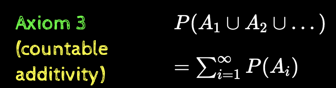
Examples

... ... ...

The third axiom that we had defined earlier was only for finite (countable) events $A1,A2,…AnA_1, A_2, \dots A_n$

We state its correct version now which accounts for infinite (countable) events $A1,A2,…AnA_1, A_2, \dots A_n$

Axiom 3 (countable additivity)

= \sum_{i=1}^\infty P(A_i)

P(A_1\cup A_2 \cup \dots )

Summary

Set Theory

Finite, Countably infinite, Uncountably infinite

Intersection, Union, Complement

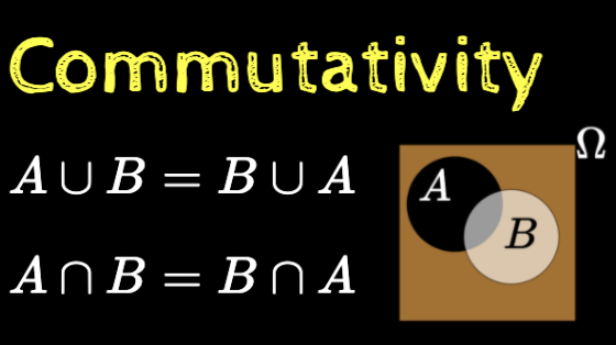
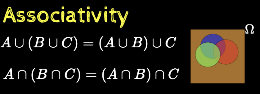
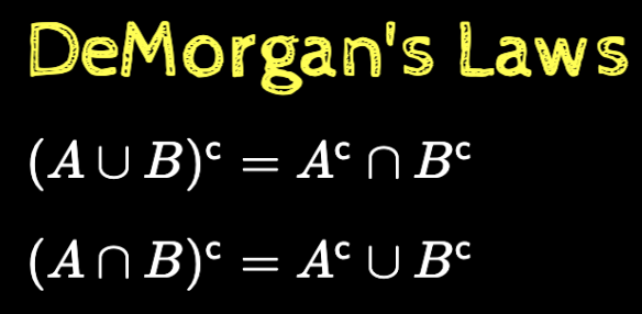
Properties of set operations

Disjoint sets

Axioms of Probability

CS6015: Linear Algebra and Random Processes

Lecture 28: Probability Space, Axioms of Probability, Designing Probability Functions

Probability Theory

Basics

Laws

Random Var.

Applications

Processes

Counting

Set Theory

Axioms

Union rule

Multiplication Rule

Total Probability Theorem

Bayes' Theorem

Independence

PMF, PDF, CDF

Expectation, Var., Moments

Distributions (~10)

Bayes' Theorem

Independence

Sampling from a distribution

Designing arbitrary probability functions

Estimating Parameters

Simple Random Walk

Bernoulli Process

Poisson Process

Markov Process

.... .... ....

Limit Theorems

Markov inequality

Chebychev inequality

Weak Law of large nos.

Central Limit Theorem

The

St

Joint, cond., marginal dist.

.... .... ....

Learning Objectives

What is a probability space?

What are the axioms of probability?

What are some simple ways of defining a probability function?

Probability Space

Definitions

\(\Omega\): Sample space (all outcomes)

Event: subsets of \(\Omega\)

Field \(\mathcal{F}\): a subcollection of the set of all subsets of \(\Omega\) such that

if \(A,B \in \mathcal{F}\) then \(A\cap B \in \mathcal{F}\) and \(A\cup B \in \mathcal{F}\)

if \(A \in \mathcal{F}\) then \(A^\mathsf{c} \in \mathcal{F}\)

\(\phi\in \mathcal{F}\)

(empty set)

Why not simply say all subsets of \(\Omega\) ?

(beyond the scope of this course)

Definitions

\(\sigma\)-field \(\mathcal{F}\): A collection of the subsets of \(\Omega\) is called a \(\sigma\)-field if

if \(A_1,A_2, \dots \in \mathcal{F}\) then \(\cup_{i=1}^{\infty} A_i \in \mathcal{F}\)

if \(A \in \mathcal{F}\) then \(A^\mathsf{c} \in \mathcal{F}\)

\(\phi\in \mathcal{F}\)

(empty set)

if \(A_1,A_2, \dots \in \mathcal{F}\) then \(\cap_{i=1}^{\infty} A_i \in \mathcal{F}\)

closed under countable unions & intersections

The power set of \(\Omega\) which contains ALL subsets of \(\Omega\) is obviously a \(\sigma\)-field

Definitions

a probability measure \(\mathbb{P}\) on \(\Omega, \mathcal{F}\) is a function \(\mathbb{P}: \mathcal{F} \rightarrow [0,1] \) satisfying the axioms of probability

The triple \((\Omega, \mathcal{F}, \mathbb{P})\) where \(\mathcal{F}\) is a \(\sigma\)-field, is called a probability space

(we will soon see what these axioms are)

Recap

Experiments

Sample Space

Events

What is the chance of an event?

Goal: Assign a number to each event such that this number reflects the chance of the experiment resulting in that event

(\(\sigma\)-field \(\mathcal{F}\))

The probability function

What are the conditions that such a probability function must satisfy?

(Axioms of Probability)

Event

Probability function

The axioms of probability

Axiom 1 (non-negativity)