CS6015: Linear Algebra and Random Processes

Lecture 35: Continuous random variables, probability mass function v/s probability density function, cumulative distribution function

Learning Objectives

What are continuous random variables?

What is a probability density function?

How is it different from a probability mass function?

What is a cumulative distribution function?

Todo: add slides on

1) arbitrary pdfs

2) Expectation and variance of continuous RVs

Continuous Random Variables

Recap

Probability Mass Function

p_X(x)

1~~~2~~~3~~~4~~~5~~~6

0.2

0.4

0.6

0.8

1.0

Cumulative Distribution Function

p_X(x)

1~~~2~~~3~~~4~~~5~~~6

0.2

0.4

0.6

0.8

1.0

F_X(x)

1~~~2~~~3~~~4~~~5~~~6

0.2

0.4

0.6

0.8

1.0

P(X \leq x)

Cumulative Distribution Function

F_X(x)

p_X(x)

P(X \leq x)

\frac{1}{36}

\frac{2}{36}

\frac{3}{36}

\frac{4}{36}

\frac{5}{36}

\frac{6}{36}

\frac{5}{36}

\frac{4}{36}

\frac{3}{36}

\frac{2}{36}

\frac{1}{36}

\frac{1}{6}

\frac{2}{6}

\frac{3}{6}

\frac{4}{6}

\frac{5}{6}

1 = \frac{6}{6}

\frac{1}{36}

\frac{3}{36}

\frac{6}{36}

\frac{10}{36}

\frac{15}{36}

\frac{21}{36}

\frac{1}{6}

\frac{2}{6}

\frac{3}{6}

\frac{4}{6}

\frac{5}{6}

1 = \frac{6}{6}

\frac{26}{36}

\frac{30}{36}

\frac{33}{36}

\frac{35}{36}

\frac{36}{36}

Recap

p_X(x)

\frac{1}{36}

\frac{2}{36}

\frac{3}{36}

\frac{4}{36}

\frac{5}{36}

\frac{6}{36}

\frac{5}{36}

\frac{4}{36}

\frac{3}{36}

\frac{1}{36}

\frac{1}{6}

\frac{2}{6}

\frac{3}{6}

\frac{4}{6}

\frac{5}{6}

1 = \frac{6}{6}

Probability Mass Function

Total Probability = 1 (unit mass)

PMF: What share of this unit mass does each value take?

What if the random variable can take infinite values?

(continuous random variables)

Continuous Random Variables

Total Probability = 1 (unit mass)

What share of the unit probability mass does each value take?

Rainfall in Chennai:

Exactly 2 cm ?

2.01, 2.001, 1.99, 1.999

0 Infinite values possible

Continuous Random Variables

Your water intake (in litres )

Does not make sense to ask about the number of days on which you drank exactly 2 litres?

Instead it makes sense to ask about the number of days on which 1.9 < x < 2.1

1.0 1.5 2.5 2.5 3.0 3.5

\Omega

last 512 days

Continuous Random Variables

Your water intake (in litres )

Instead it makes sense to ask about the number of days on which 1.9 < x < 2.1

1.0 1.5 2.0 2.5 3.0 3.5

Continuous Random Variables

Your water intake (in litres )

1.0 1.5 2.0 2.5 3.0 3.5

probability density function

cumulative distribution function

probability mass function

cumulative distribution function

p_X(x) \geq 0

P(a \leq X \leq b) = \sum_{x=a}^b p_X(x)

f_X(x) \geq 0

P(a \leq X \leq b) = \int_{a}^b f_X(x) dx

\int_{-\infty}^\infty f_X(x) dx = 1

\sum_x p_x(x) = 1

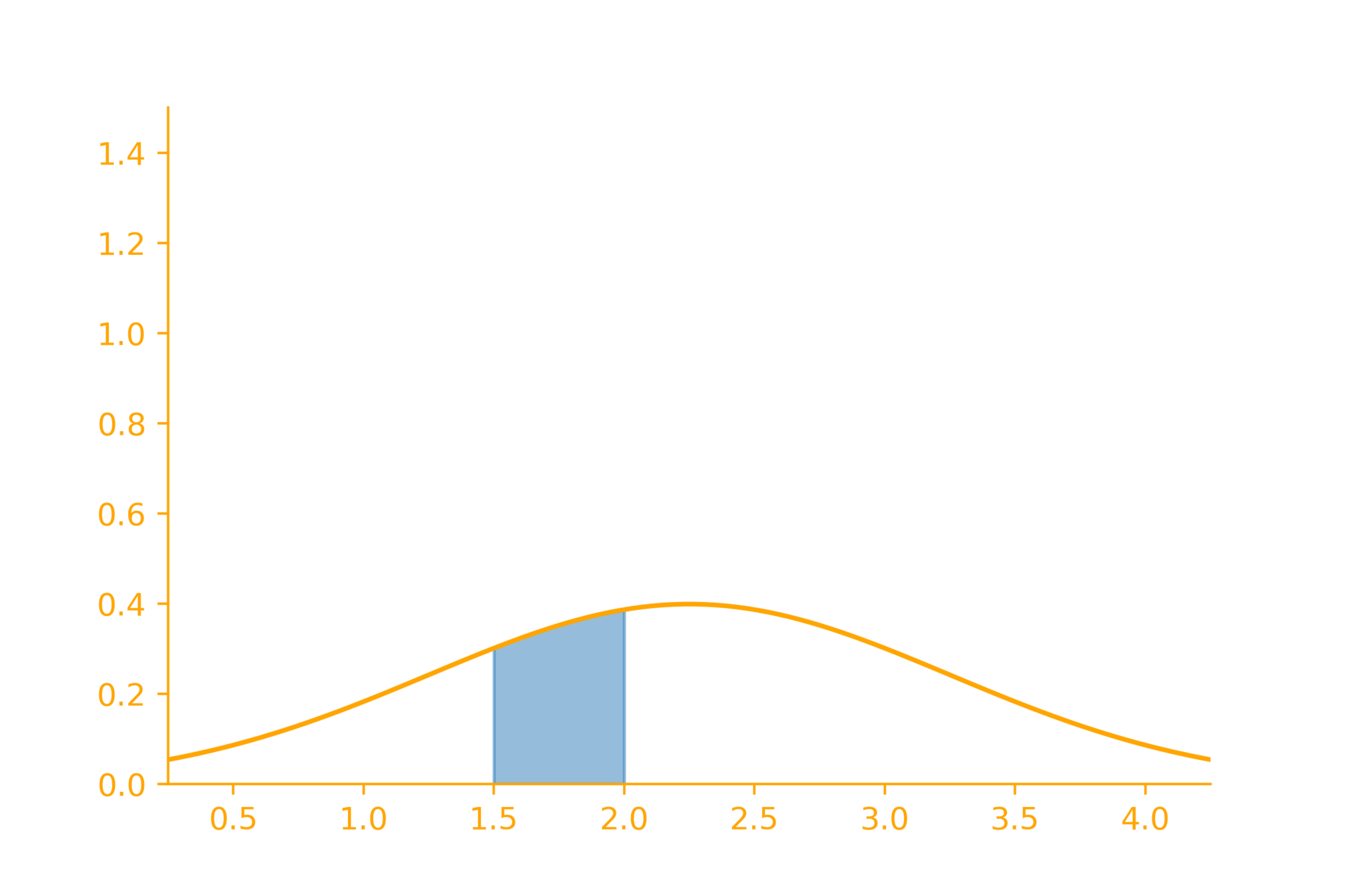
Intuition: Density v/s Mass

probability density function

probability mass function

\delta

f_X(x)

P_X(a\leq x \leq a + \delta) = f_X(x)\cdot \delta

Summary

For continuous random variables

P(X=x) = 0 \forall x

Questions of interest are

P(a\leq X \leq b)

pdf does not directly give us probability

(probability of an interval is obtained by integrating over that interval)

P_X(a\leq x \leq a + \delta) \approx f_X(x)\cdot \delta

Properties of pdf

f_X(x)\geq 0

\int_{-\infty}^\infty f_X(x) dx = 1

Learning Objectives

What are continuous random variables?

What is a probability density function?

How is it different from a probability mass function?

What is a cumulative distribution function?

Todo: add slides on

1) arbitrary pdfs

2) Expectation and variance of continuous RVs

Uniform distribution (continuous)

Discrete Uniform Distribution

\frac{1}{b - a}

p_X(x)

f_X(x)

Continuous Uniform Distribution

a_1

b_1

[

]

P(a_1 \leq X \leq b_1) = \frac{1}{b-a} (b_1 - a_1)

\dots

\frac{1}{b - a + 1}

Expectation

f_X(x)

p_X(x)

\dots

\frac{1}{b - a + 1}

E[X] = \sum_x xp_X(x)

E[g(X)] = \sum_x g(x) p_X(x)

Var(X) = E[X^2] - (E[X])^2

E[X] = \int_{-\infty}^{\infty} xf_X(x) dx

E[g(X)] = \int_{-\infty}^{\infty}g(x) p_X(x)dx

Var(X) = E[X^2] - (E[X])^2

Mean and variance (Uniform Distribution)

E[X] = \int_{a}^{b} x\frac{1}{b-a} dx

E[g(X)] = \int_{-\infty}^{\infty}g(x) p_X(x) dx

Var(X) = E[X^2] - (E[X])^2

\frac{1}{b - a}

f_X(x)

=\frac{a+b}{2}

E[X] = \int_{-\infty}^{\infty} xf_X(x) dx

E[X^2] = \int_{a}^{b} x^2\frac{1}{b-a} dx

=\frac{1}{b-a}(\frac{b^3}{3} - \frac{a^3}{3})

Var(X) = E[X^2] - (E[X])^2 = \frac{(b-a)^2}{12}

E[X] = \int_{a}^{b} x\frac{1}{b-a} dx

E[X^2] = \int_{a}^{b} x^2\frac{1}{b-a} dx

E[X] =\frac{1}{b-a} * \frac{x^2}{2} |_{a}^b

= \frac{1}{b-a} * (\frac{b^2}{2} - \frac{a^2}{2}) = \frac{1}{b-a}\frac{b^2 - a^2}{2}

= \frac{1}{b-a}\frac{(b - a)(b+a)}{2} = \frac{a+b}{2}

=\frac{1}{b-a} * \frac{x^3}{3} |_{a}^b

= \frac{1}{b-a} * (\frac{b^3}{3} - \frac{a^3}{3}) = \frac{1}{b-a}\frac{b^3 - a^3}{3}

= \frac{1}{b-a}\frac{(b - a)(a^2 + ab + b^2)}{3} = \frac{a^2 + ab + b^2}{3}

Var(X) = E[X^2] - E[X]^2

= \frac{a^2 + ab + b^2}{3} - (\frac{a+b}{2})^2

= \frac{a^2 + ab + b^2}{3} - \frac{a^2 + 2ab + b^2}{4}

= \frac{(b-a)^2}{12}

Normal Distribution

Some fun with functions

x^2

e^x

e^{-x}

e^{x^2}

e^{-x^2}

20 * e^{-x^2}

Some fun with functions

e^{-x^2}

Normal distribution

\mathcal{N}(0, 1) = \frac{1}{\sqrt{2 \pi}}e^{-x^2}

\int_{-\infty}^{\infty} \frac{1}{\sqrt{2 \pi}}e^{-x^2} dx = 1

Normal distribution

\mathcal{N}(0, 1) = \frac{1}{\sqrt{2 \pi}}e^{-x^2}

E[X] = \int_{-\infty}^{\infty}x\cdot\frac{1}{\sqrt{2 \pi}}e^{-x^2} dx

= 0

Var[X] = E[X^2] - (E[X])^2

= 1

zero mean, unit variance

\mu = 0, \sigma = 1

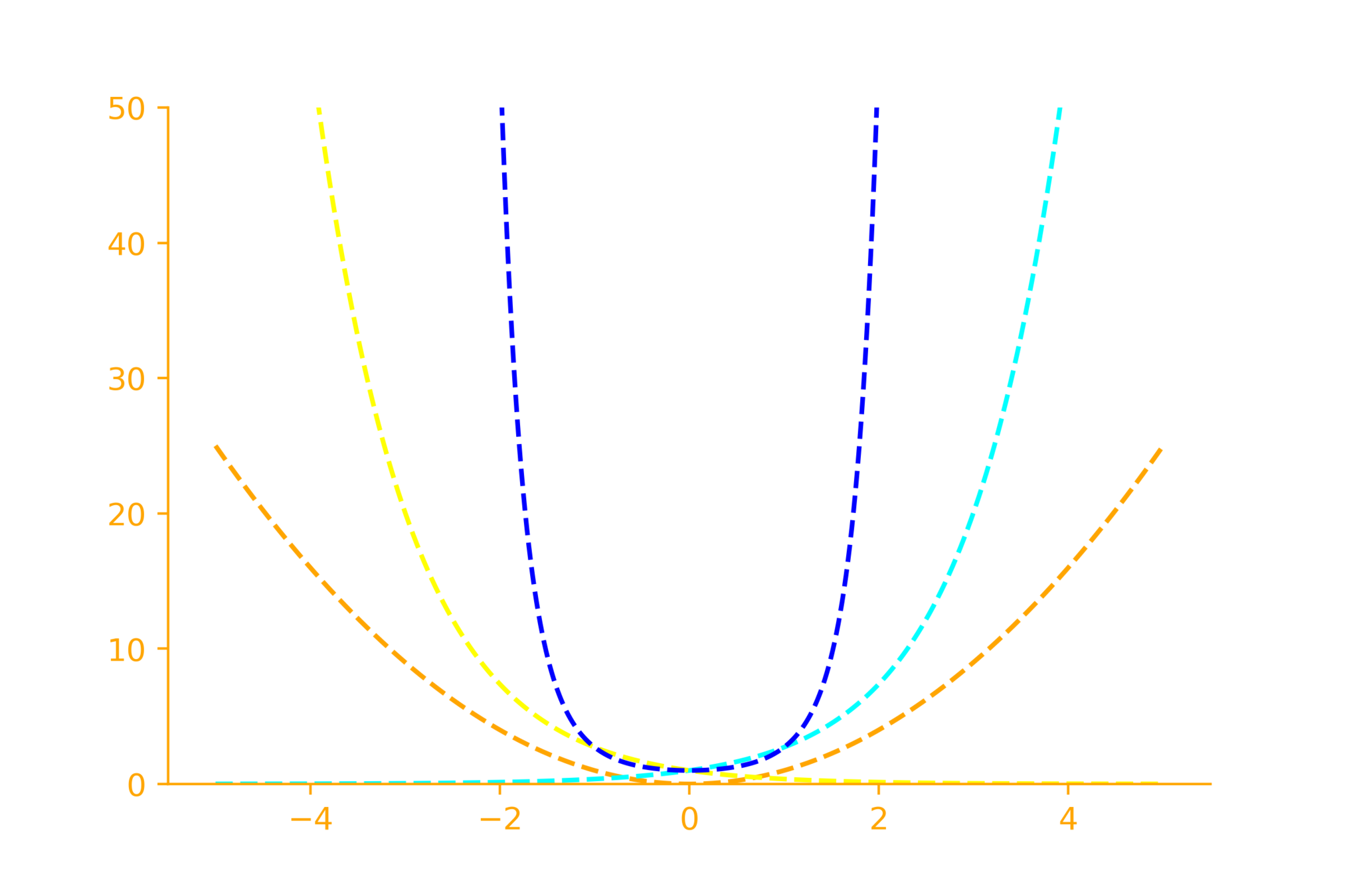
Normal distribution (changing

\mathcal{N}(\mu, 1) = \frac{1}{\sqrt{2 \pi}}e^{-\frac{(x-\mu)^2}{2}}

E[X] = \int_{-\infty}^{\infty}x\cdot\frac{1}{\sqrt{2 \pi}}e^{-\frac{(x-\mu)^2}{2}} dx

= \mu

Var[X] = E[X^2] - (E[X])^2

= 1

\mu = 2

\mu = 0

\mu = -2

\mu)

Normal distribution (changing

\mathcal{N}(0, \sigma^2) = \frac{1}{\sqrt{2 \pi}}e^{\frac{-x^2}{2\sigma^2}}

E[X] = \int_{-\infty}^{\infty}x\cdot\frac{1}{\sqrt{2 \pi}}e^{\frac{-x^2}{2\sigma^2}} dx

= 0

Var[X] = E[X^2] - (E[X])^2

= \sigma^2

\sigma = 0.5

\sigma = 1

\sigma = 2

\sigma)

Normal distribution (changing

\mathcal{N}(\mu, \sigma^2) = \frac{1}{\sqrt{2 \pi}}e^{\frac{-(x-\mu)^2}{2\sigma^2}}

E[X] = \int_{-\infty}^{\infty}x\cdot\frac{1}{\sqrt{2 \pi}}e^{\frac{-(x-\mu)^2}{2\sigma^2}} dx

= \mu

Var[X] = E[X^2] - (E[X])^2

\mu = 2, \sigma = 0.5

\mu, \sigma)

= \sigma^2

The distribution is fully specified by the parameters:

\mu, \sigma^2

Normal distribution

\sigma

68\%

95\%

99\%

P(\mu - \sigma \leq X \leq \mu + \sigma)

= \int_{\mu - \sigma}^{\mu + \sigma} \frac{1}{\sqrt{2\pi}} e^{ \frac{-(x - \mu)}{2 \sigma^2} } dx

\approx 0.68

P(\mu - 2\sigma \leq X \leq \mu + 2\sigma)

= \int_{\mu - 2\sigma}^{\mu + 2\sigma} \frac{1}{\sqrt{2\pi}} e^{ \frac{-(x - \mu)}{2 \sigma^2} } dx

\approx 0.95

Sampling Methods

Recap

A population is the total collection of all objects that we are interested in studying

A sample is a subgroup of the population that we study to draw inferences about the population

Population

Sample

Question: How do we select these samples?

(Let' start with some wrong ways of selecting samples)

Biased Samples

Convenience Sample

Voluntary Sample

(non-response bias)

Convenience Samples

Goal: Compute average height of students

Convenience Sample: Take the students sitting on the first bench so that you don't disturb the whole class

Bias: Shorter students sit on the first bench

Convenience Samples

Goal: Compute prevalence of COVID-19

Convenience Sample: Just consider people who are visiting ENT hospitals instead of sending out a collection team

Bias: People visiting ENT hospitals may include a higher proportion of infected people

Flu

\Omega

Convenience Samples

Goal: Predict results of presidential polls (1948)

Convenience Sample: Conduct surveys on phones

Bias: Only richer people had phones in 1948

\Omega

Convenience Samples

Goal: Draft citizens into military

Bias: People born in December were getting drafted more than others

Convenience Sample: Put the numbers 1 to 366 in a jar and then draw a number

Voluntary Samples

Goal: Predict results of presidential polls (1936)

Voluntary Sample: 1M Postal survey forms were sent to people of which 24% responded

Bias: More Republican voters responded as compared to Democratic voters

Voluntary Samples

A voluntary bias or non-response bias occurs when people who respond/participate are very different from those who do not

Voluntary Samples

Goal: Predict proportion of people who are favourable

Voluntary Sample: Check social media posts

Bias: Disgruntled citizens are more likely to post as compared to citizens who are happy with the policy

A sample that is representative of the entire population and gives each element an equal chance of being chosen

Unbiased Samples

Convenience sampling

Sampling Strategies

Simple random sampling

Systematic sampling

Cluster sampling

Stratified sampling

Convenience sampling

Sampling Strategies

Simple random sampling

Systematic sampling

Cluster sampling

Stratified sampling

import numpy as np
low = 1 //start
high = 72 //total_population
size = 9 //sample_size

np.random.randint(low, high, size)

Experimental Studies

Experiment

Apply treatment to experimental units and make observations to compare treatments

Example

Dr. Watson wants to study the effect of quantity (4-10) and type of nuts (almond, walnuts, cashews) on cholesterol levels of heart patients.

Response variable:

Cholesterol level

Experimental unit:

Heart patients

Factors:

Quantity

Factor Levels:

4 - 10

almond, walnut, cashew

Type of nuts

Treatment:

Combination of factor levels

Lurking variables:

Age, Diet, Exercise

Example

12 Treatments:

Combinations of factor levels

Lurking variables:

Age, Diet, Exercise

4

6

8

10

Experiments: Basic Principles

Randomization

Subjects are assigned randomly to treatment groups

Repetition

Control

Multiple subjects are given the same treatment

Control the effect of lurking variables

Placebo Effect

Actual Treatment

Experimental Group

Empty Pills

Control Group

(placebo)

Lurking variables:

Sleep, Diet, Exercise

(same sleep time, diet and exercise routine for both groups)

Single Blind Experiment

Double Blind Experiment

Subjects don't know which group they are in

Both experimenter and subjects don't know which group is which

Types of Experiment Designs

Completely Randomized Designs

Block Randomized Designs

Males

Females

Types of Experiment Designs

Matched Pair Design

Fuel A

Fuel B

Compare

Fuel A

Fuel B

Compare

Fuel A

Fuel B

Compare

Fuel A

Fuel B

Compare

Apply all treatments to same/similar objects

Types of Experiment Designs

Matched Pair Design

Apply all treatments to same/similar objects

Does sleep deprivation affect performance on a test?

Key Terms and Definitions

In Statistics we are always, interested in studying a large collection of people or objects

Opinion Poll: What proportion of the citizens support candidate XYZ ?

Challenge: Infeasible (expensive) to survey all citizens

In Statistics we are always, interested in studying a large collection of people or objects

Car Testing: What is the average mileage of cars produced in a factory?

Challenge: Expensive to test all cars

Key Terms and Definitions

Randomness everywhere!

How many infections in the neighbourhood?

Examples

If he does not come out alive what is the probability that he took path A1?

P(A_1|B) = ?

B : monster encountered

i-th path taken

A_i:

P(A_1|B) = \frac{P(A_1 \cap B)}{P(B)}

P(A_1|B) = \frac{P(A_1 \cap B)}{P(A_1)\cdot P(B|A_1) + P(A_2)\cdot P(B|A_2) + P(A_3)\cdot P(B|A_3)}

P(A_1 \cap B) = P(A_1)P(B|A_1) \\ P(A_1 \cap B) = P(B)P(A_1|B)

P(A_1)=P(A_2)=P(A_3) = \frac{1}{3}

P(B|A_1) = 0.3

P(B|A_2) = 0.6

P(B|A_3) = 0.75