Curso-Taller

!Bienvenidos!

Dia 1: Introducción

Que es julia
Porque julia
Instalación y entornos de desarrollo
Literatura disponible
Ecosistema

Que es julia

Origen:

El lenguaje fue creado por Stefan Karpinski, estudiante graduado de la Universidad de California, que estaba involucrado en una herramienta simulación de redes que requería el uso de varios lenguajes de programación diferentes. Curiosamente, ninguno de los lenguajes usados podía hacer toda la tarea, todo el proceso. Por ello, Karpinski, junto con su compañero de universidad Viral Shah y Jeff Bezanson del MIT, decidieron resolverlo diseñando un nuevo lenguaje que fuera compatible con prácticamente cualquier tarea. La meta de Karpinski y su equipo es construir un lenguaje único que haga todo bien.

Julia es un lenguaje de programación multiplataforma y multiparadigma de tipado dinámico de alto nivel y alto desempeño para la computación genérica, técnica y científica, con una sintaxis similar a la de otros lenguajes de programación.

Dispone de un compilador avanzado (JIT), mecanismos para la ejecución en paralelo y distribuida, ademas de una extensa biblioteca de funciones matemáticas desarrollada fundamentalmente en Julia, y también contiene código desarrollado en C y Fortran para el álgebra lineal, generación de números aleatorios, procesamiento de señales, procesamiento de cadenas,entre otros.

Porque julia

El nombre:

El nombre del lenguaje Julia fue puesto en honor a Gaston Julia, un matematico frances que descubrio los fractales.

Usarlo:

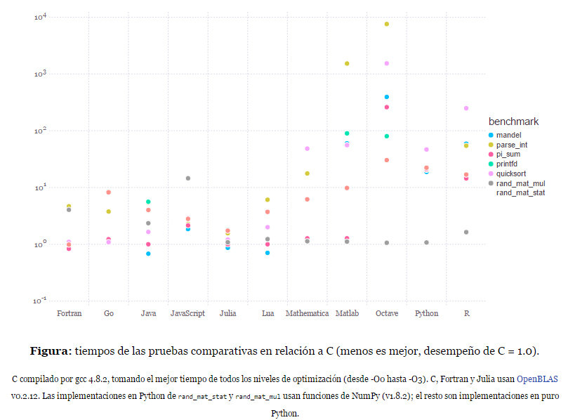
Tanto el compilador justo a tiempo (JIT) basado en LLVM así como el diseño del lenguaje le permiten a Julia acercarse e incluso igualar a menudo el desempeño de C. Los resultados de las siguientes micro pruebas comparativas se obtuvieron usando un Intel(R) Xeon(R) CPU de un solo núcleo (ejecución serial) E7-8850 2.00GHz CPU con 1TB de 1067MHz DDR3 RAM, corriendo en Linux:

La version:

Instalación y entornos de desarrollo

Ubuntu:
    sudo add-apt-repository ppa:staticfloat/juliareleases
    sudo add-apt-repository ppa:staticfloat/julia-deps
    sudo apt-get update
    sudo apt-get install julia
Fedora: 
    sudo dnf copr enable nalimilan/julia
    sudo yum install julia

Varias opciones:

a)Binarios: vamos a http://julialang.org/downloads/
b)Manejador de paquetes

c)Compilacion del codigo fuente

https://github.com/JuliaLang/julia

d)IJulia: usar julia en el

navegador web

e)Uso en linea

$ julia
               _
   _       _ _(_)_     |  A fresh approach to technical computing
  (_)     | (_) (_)    |  Documentation: http://docs.julialang.org
   _ _   _| |_  __ _   |  Type "?help" for help.
  | | | | | | |/ _` |  |
  | | |_| | | | (_| |  |  Version 0.4.0-dev+6859 (2015-08-20 19:38 UTC)
 _/ |\__'_|_|_|\__'_|  |  Commit 92ddae7 (55 days old master)
|__/                   |  x86_64-w64-mingw32

julia> println("hello world")

Instalación y entornos de desarrollo

Vim: julia-vim
Emacs: marcado de la sintaxis de julia gracias a este paquete.
Sublime Text: Sublime-IJulia integra a IJulia dentro Sublime Text -la instalacion es algo compleja pero vale la pena.
Notepad++: soporte de la sintaxis mediante un archivo de configuracion
Light Table: soporte a Julia mediante el proyecto Juno (solo hasta la version 0.3.11).
Atom: Ide oficial para la version 0.4

Literatura disponible

Ecosistema

Día 2: Instrucciones básicas

Aritmética enteros, Flotantes, complejos
Variables
Condicionales
Iteraciones
Funciones matemáticas
Funciones

Aritmetica

Variables

julia> m = 2.32
    2.32 

julia> m
    2.32

julia> ❄ = -12
    -12

julia> ✹ = 27
    27

julia> ❄ > ✹
    false

julia> π
   π = 3.1415926535897...

julia> π = 3.2
  Warning: imported binding for π overwritten in module Main
    3

julia> π
    3.2

Condicionales

Iteraciones

Funciones matematicas

function sphere_vol(r)
    # julia allows Unicode names (in UTF-8 encoding)
    # so either "pi" or the symbol π can be used
    return 4/3*pi*r^3
end

# functions can also be defined more succinctly
quadratic(a, sqr_term, b) = (-b + sqr_term) / 2a

# calculates x for 0 = a*x^2+b*x+c, arguments types can be defined in function definitions
function quadratic2(a::Float64, b::Float64, c::Float64)
    # unlike other languages 2a is equivalent to 2*a
    # a^2 is used instead of a**2 or pow(a,2)
    sqr_term = sqrt(b^2-4a*c)
    r1 = quadratic(a, sqr_term, b)
    r2 = quadratic(a, -sqr_term, b)
    # multiple values can be returned from a function using tuples
    # if the return keyword is omitted, the last term is returned
    r1, r2
end

vol = sphere_vol(3)
# @printf allows number formatting but does not automatically append the \n to statements, see below
@printf "volume = %0.3f\n" vol 
#> volume = 113.097

quad1, quad2 = quadratic2(2.0, -2.0, -12.0)
println("result 1: ", quad1)
#> result 1: 3.0
println("result 2: ", quad2)
#> result 2: -2.0

Funciones

Día 3: Estructuras de datos

Arreglos
cadenas
colecciones
diccionarios
tuplas
matrices y álgebra lineal
Tipos de datos

ARREGLOS

function printsum(a)
    # summary generates a summary of an object
    println(summary(a), ": ", repr(a))
end

# arrays can be initialised directly:
a1 = [1,2,3]
printsum(a1)
#> 3-element Array{Int64,1}: [1,2,3]

# or initialised empty:
a2 = []
printsum(a2)
#> 0-element Array{None,1}: None[]

# since this array has no type, functions like push! (see below) don't work
# instead arrays can be initialised with a type:
a3 = Int64[]
printsum(a3)
#> 0-element Array{Int64,1}: []

# ranges are different from arrays:
a4 = 1:20
printsum(a4)
#> 20-element UnitRange{Int64}: 1:20

# however they can be used to create arrays thus:
a4 = [1:20]
printsum(a4)
#> 20-element Array{Int64,1}: [1,2,3,4,5,6,7,8,9,10,11,12,13,14,15,16,17,18,19,20]

# arrays can also be generated from comprehensions:
a5 = [2^i for i = 1:10]
printsum(a5)
#> 10-element Array{Int64,1}: [2,4,8,16,32,64,128,256,512,1024]

# arrays can be any type, so arrays of arrays can be created:
a6 = (Array{Int64, 1})[]
printsum(a6)
#> 0-element Array{Array{Int64,1},1}: []
# (note this is a "jagged array" (i.e., an array of arrays), not a multidimensional array, these are not covered here)

# Julia provided a number of "Dequeue" functions, the most common for appending to the end of arrays is push!
# ! at the end of a function name indicates that the first argument is updated.

push!(a1, 4)
printsum(a1)
#> 4-element Array{Int64,1}: [1,2,3,4]

# push!(a2, 1) would cause error:

push!(a3, 1)
printsum(a3) #> 1-element Array{Int64,1}: [1]
#> 1-element Array{Int64,1}: [1]

push!(a6, [1,2,3])
printsum(a6)
#> 1-element Array{Array{Int64,1},1}: [[1,2,3]]

# using repeat() to create arrays
# you must use the keywords "inner" and "outer"
# all arguments must be arrays (not ranges)
a7 = repeat(a1,inner=[2],outer=[1])
printsum(a7)
#> 8-element Array{Int64,1}: [1,1,2,2,3,3,4,4]
a8 = repeat([4:-1:1],inner=[1],outer=[2])
printsum(a8)
#> 8-element Array{Int64,1}: [4,3,2,1,4,3,2,1]

Caracteres

julia> 'x'
'x'

julia> typeof(ans)
Char

julia> Int('x')
120

julia> typeof(ans)
Int64

julia> Char(120)
'x'

julia> Int('\0')
0

julia> Int('\t')
9

julia> Int('\n')
10

# strings are defined with double quotes
# like variables, strings can contain any unicode character
s1 = "The quick brown fox jumps over the lazy dog α,β,γ"
println(s1)
#> The quick brown fox jumps over the lazy dog α,β,γ

# println adds a new line to the end of output
# print can be used if you dont want that:
print("this")
#> this
print(" and")
#> and
print(" that.\n")
#> that.

# chars are defined with single quotes
c1 = 'a'
println(c1)
#> a
# the ascii value of a char can be found with int():
println(c1, " ascii value = ", int(c1))
#> a ascii value = 97
println("int('α') == ", int('α'))
#> int('α') == 945

# so be aware that
println(int('1') == 1)
#> false

# strings can be converted to upper case or lower case:
s1_caps = uppercase(s1)
s1_lower = lowercase(s1)
println(s1_caps, "\n", s1_lower)
#> THE QUICK BROWN FOX JUMPS OVER THE LAZY DOG Α,Β,Γ
#> the quick brown fox jumps over the lazy dog α,β,γ

# sub strings can be indexed like arrays:
# (show prints the raw value)
show(s1[11]); println()
#> 'b'

# or sub strings can be created:
show(s1[1:10]); println()
#> "The quick "

# end is used for the end of the array or string
show(s1[end-10:end]); println()
#> "dog α,β,γ"

# julia allows string Interpolation:
a = "wolcome"
b = "julia"
println("$a to $b.")
#> wolcome to julia.

# this can extend to evaluate statements:
println("1 + 2 = $(1 + 2)")
#> 1 + 2 = 3

# strings can also be concatenated using the * operator
# using * instead of + isn't intuitive when you start with Julia,
# however people think it makes more sense
s2 = "this" * " and" * " that"
println(s2)
#> this and that

# as well as the string function
s3 = string("this", " and", " that")
println(s3)
#> this and that

CADENAS

Cadenas: Conversion y formato

# strings can be converted using float and int:
e_str1 = "2.718"
e = float(e_str1)
println(5e)
#> 13.5914
num_15 = int("15")
println(3num_15)
#> 45

# numbers can be converted to strings and formatted using printf
@printf "e = %0.2f\n" e
#> 2.718
# or to create another string sprintf
e_str2 = @sprintf("%0.3f", e)

# to show that the 2 strings are the same
println("e_str1 == e_str2: $(e_str1 == e_str2)")
#> e_str1 == e_str2: true

# available number format characters are f, e, g, c, s, p, d:
# (pi is a predefined constant; however, since its type is 
# "MathConst" it has to be converted to a float to be formatted)
@printf "fix trailing precision: %0.3f\n" float(pi)
#> fix trailing precision: 3.142
@printf "scientific form: %0.6e\n" 1000pi
#> scientific form: 3.141593e+03
# g is not implemented yet
@printf "a character: %c\n" 'α'
#> a character: α
@printf "a string: %s\n" "look I'm a string!"
#> a string: look I'm a string!
@printf "right justify a string: %50s\n" "width 50, text right justified!"
#> right justify a string:                    width 50, text right justified!
@printf "a pointer: %p\n" 1e10
#> a pointer: 0x00000002540be400
@printf "print a integer: %d\n" 1e10
#> print an integer: 10000000000

Cadenas: Manipulaciones

s1 = "The quick brown fox jumps over the lazy dog α,β,γ"

# search returns the first index of a char
i = search(s1, 'b')
println(i)
#> 11
# the second argument is equivalent to the second argument of split, see below

# or a range if called with another string
r = search(s1, "brown")
println(r)
#> 11:15


# string replace is done thus:
r = replace(s1, "brown", "red")
show(r); println()
#> "The quick red fox jumps over the lazy dog"

# search and replace can also take a regular expressions by preceding the string with 'r'
r = search(s1, r"b[\w]*n")
println(r)
#> 11:15

# again with a regular expression
r = replace(s1, r"b[\w]*n", "red")
show(r); println()
#> "The quick red fox jumps over the lazy dog"

# there are also functions for regular expressions that return RegexMatch types
# match scans left to right for the first match (specified starting index optional)
r = match(r"b[\w]*n", s1)
println(r)
#> RegexMatch("brown")

# RegexMatch types have a property match that holds the matched string
show(r.match); println()
#> "brown"

# matchall returns a vector with RegexMatches for each match
r = matchall(r"[\w]{4,}", s1)
println(r)
#> SubString{UTF8String}["quick","brown","jumps","over","lazy"]

# eachmatch returns an iterator over all the matches
r = eachmatch(r"[\w]{4,}", s1)
for(i in r) print("\"$(i.match)\" ") end
println()
#> "quick" "brown" "jumps" "over" "lazy" 

# a string can be repeated using the repeat function, 
# or more succinctly with the ^ syntax:
r = "hello "^3
show(r); println() #> "hello hello hello "

# the strip function works the same as python:
# e.g., with one argument it strips the outer whitespace
r = strip("hello ")
show(r); println() #> "hello"
# or with a second argument of an array of chars it strips any of them;
r = strip("hello ", ['h', ' '])
show(r); println() #> "ello"
# (note the array is of chars and not strings)

# similarly split works in basically the same way as python:
r = split("hello, there,bob", ',')
show(r); println() #> ["hello"," there","bob"]
r = split("hello, there,bob", ", ")
show(r); println() #> ["hello","there,bob"]
r = split("hello, there,bob", [',', ' '], 0, false)
show(r); println() #> ["hello","there","bob"]
# (the last two arguements are limit and include_empty, see docs)

# the opposite of split: join is simply
r= join([1:10], ", ")
println(r) #> 1, 2, 3, 4, 5, 6, 7, 8, 9, 10

function Regex(pattern::AbstractString, flags::AbstractString)
    options = DEFAULT_COMPILER_OPTS
    for f in flags
        options |= f=='i' ? PCRE.CASELESS  :
                   f=='m' ? PCRE.MULTILINE :
                   f=='s' ? PCRE.DOTALL    :
                   f=='x' ? PCRE.EXTENDED  :
                   throw(ArgumentError("unknown regex flag: $f"))
    end
    Regex(pattern, options, DEFAULT_MATCH_OPTS)
end

a=4
Regex("$a dogs", "mi")

colecciones

diccionarios

# dicts can be initialised directly:
a1 = {1=>"one", 2=>"two"}
printsum(a1) #> Dict{Any,Any}: {2=>"two",1=>"one"}

# then added to:
a1[3]="three"
printsum(a1) #> Dict{Any,Any}: {2=>"two",3=>"three",1=>"one"}
# (note dicts cannot be assumed to keep their original order)

# dicts may also be created with the type explicitly set
a2 = Dict{Int64, String}()
a2[0]="zero"

# dicts, like arrays, may also be created from comprehensions
a3 = {i => @sprintf("%d", i) for i = 1:10}
printsum(a3)#> Dict{Any,Any}: {5=>"5",4=>"4",6=>"6",7=>"7",2=>"2",10=>"10",9=>"9",8=>"8",3=>"3",1=>"1"}

# as you would expect, Julia comes with all the normal helper functions
# for dicts, e.g., (haskey)[http://docs.julialang.org/en/latest/stdlib/base/#Base.haskey]
println(haskey(a1,1)) #> true

# which is equivalent to
println(1 in keys(a1)) #> true
# where keys creates an iterator over the keys of the dictionary

# similar to keys, (values)[http://docs.julialang.org/en/latest/stdlib/base/#Base.values] get iterators over the dict's values:
printsum(values(a1)) #> ValueIterator{Dict{Any,Any}}: ValueIterator{Dict{Any,Any}}({2=>"two",3=>"three",1=>"one"})

# use collect to get an array:
printsum(collect(values(a1)))#> 3-element Array{Any,1}: {"two","three","one"}

Matrices

# repeat can be useful to expand a grid
# as in R's expand.grid() function:

m1 = hcat(repeat([1:2],inner=[1],outer=[3*2]),
          repeat([1:3],inner=[2],outer=[2]),
          repeat([1:4],inner=[3],outer=[1]))
printsum(m1)
#> 12x3 Array{Int64,2}: [1 1 1
#>  2 1 1
#>  1 2 1
#>  2 2 2
#>  1 3 2
#>  2 3 2
#>  1 1 3
#>  2 1 3
#>  1 2 3
#>  2 2 4
#>  1 3 4
#>  2 3 4]

# for simple repetitions of arrays,
# use repmat
m2 = repmat(m1,1,2)     # replicate a9 once into dim1 and twice into dim2
println("size: ", size(m2))
#> size: (12,6)

m3 = repmat(m1,2,1)     # replicate a9 twice into dim1 and once into dim2
println("size: ", size(m3))
#> size: (24,3)

# Julia comprehensions are another way to easily create 
# multidimensional arrays

m4 = [i+j+k for i=1:2, j=1:3, k=1:2] # creates a 2x3x2 array of Int64
m5 = ["Hi Im # $(i+2*(j-1 + 3*(k-1)))" for i=1:2, j=1:3, k=1:2] # expressions are very flexible
# you can specify the type of the array by just 
# placing it in front of the expression
m5 = ASCIIString["Hi Im element # $(i+2*(j-1 + 3*(k-1)))" for i=1:2, j=1:3, k=1:2]
printsum(m5)
#> 2x3x2 Array{ASCIIString,3}: ASCIIString["Hi Im element # 1" "Hi Im element # 3" "Hi Im element # 5"
#>             "Hi Im element # 2" "Hi Im element # 4" "Hi Im element # 6"]
#> 
#> ASCIIString["Hi Im element # 7" "Hi Im element # 9" "Hi Im element # 11"
#>             "Hi Im element # 8" "Hi Im element # 10" "Hi Im element # 12"]

# Array reductions
# many functions in Julia have an array method
# to be applied to specific dimensions of an array:

sum(m4,3)        # takes the sum over the third dimension
sum(m4,(1,3)) # sum over first and third dim

maximum(m4,2)    # find the max elt along dim 2
findmax(m4,3)    # find the max elt and its index along dim 2 (available only in very recent Julia versions)

# Broadcasting
# when you combine arrays of different sizes in an operation,
# an attempt is made to "spread" or "broadcast" the smaller array
# so that the sizes match up. broadcast operators are preceded by a dot: 

m4 .+ 3       # add 3 to all elements
m4 .+ [1:2]      # adds vector [1,2] to all elements along first dim

# slices and views
m4[:,:,1]  # holds dim 3 fixed and displays the resulting view
m4[:,2,:]  # that's a 2x1x2 array. not very intuititive to look at

# get rid of dimensions with size 1:
squeeze(m4[:,2,:],2)  # that's better

# assign new values to a certain view
m4[:,:,1] = rand(1:6,2,3)
printsum(m4)
#> 2x3x2 Array{Int64,3}: [3 5 2
#>  2 2 2]
#> 
#> [4 5 6
#>  5 6 7]

# (for more examples of try, catch see Error Handling above)
try
    # this will cause an error, you have to assign the correct type
    m4[:,:,1] = rand(2,3)
catch err
    println(err)
end
#> InexactError()

try
    # this will cause an error, you have to assign the right shape
    m4[:,:,1] = rand(1:6,3,2)
catch err
    println(err)
end
#> DimensionMismatch("tried to assign 3x2 array to 2x3x1 destination")

algebra lineal

Tipos de datos

type Person
    name::String
    male::Bool
    age::Float64
    children::Int
end

p = Person("Julia", false, 4, 0)
printsum(p)
#> Person: Person("Julia",false,4.0,0)

people = Person[]
push!(people, Person("Steve", true, 42, 0))
push!(people, Person("Jade", false, 17, 3))
printsum(people)
#> 2-element Array{Person,1}: [Person("Steve",true,42.0,0),Person("Jade",false,17.0,3)]

# types may also contains arrays and dicts
# constructor functions can be defined to easily create objects
type Family
    name::String
    members::Array{String, 1}
    extended::Bool
    # constructor that takes one argument and generates a default
    # for the other two values
    Family(name::String) = new(name, String[], false)
    # constructor that takes two arguements and infers the third
    Family(name::String, members) = new(name, members, length(members) > 3)
end

fam1 = Family("blogs")
println(fam1)
#> Family("blogs",String[],false)
fam2 = Family("jones", ["anna", "bob", "charlie", "dick"])
println(fam2)

Día 4: I/O y paradigmas de programación

Entrada-salida estándar
Manejo de archivos
Meta programación
Paradigma funcional

Entrada-salida estandar

manejo de archivos

Metaprogramacion

julia> e = 
:(
    for i in 1:10
        println(i)
    end
)

:(for i = 1:10 # line 2:
    println(i)
end)

julia> eval(e)
1
2
3
4
5
6
7
8
9
10

Día 5: Complementos del lenguaje

Paquetes
Procesamiento paralelo
Base de datos
Graficacion
Calculo diferencial e Integral
Ecuaciones diferenciales
Métodos numéricos
Estructura de datos
Interfaz con otros lenguajes