Fusion Energy Neutronics Workshop
This work was funded by the RCUK Energy Programme
[Grant number EP/P012450/1]
Neutron creation
(n,n')
(n,f)
(n,n')
(γ,γ')
(n,nγ')
(n,pn')
(n,f)
(n,2n)
(n,α)
(n,γ)

Cerberus
Nuclear


How can neutronics help
Radioactivity - Neutrons activate material, making it radioactive leading to handling and waste storage requirements.

Hazardous - Neutrons are Hazardous to health and shielded will be needed to protect the workforce.
Produce fuel - Neutrons will be needed to convert lithium into tritium to fuel the reactor.
Electricity - 80% of the energy release by each DT reaction is transferred to the neutron.
Structural integrity - Neutrons cause damage to materials such as embrittlement, swelling, change conductivity …

Diagnose - Neutrons are an important method of measuring a variety of plasma parameters (e.g. Q value).

Topics Covered

Material
Geometry
Tally
Source
- Cross sections


- Materials
Li4SiO4, lithium lead, tungsten
- Particle sources (point source, plasma, gamma)
- Geometry (CSG and CAD)

- Tallies (TBR, heat, spectra, dose, DPA)

- Tally types (cell, mesh, surface)
- Parameter studies

How to get setup
- Install Docker
- Download the docker image
- Run the docker image
- Navigate to the URL in the terminal
- Install Paraview and Freecad


Instructions are on the Github repository along with a setup video


docker run -p 8888:8888 ghcr.io/fusion-energy/neutronics-workshopdocker pull ghcr.io/fusion-energy/neutronics-workshopWhat are the tasks like
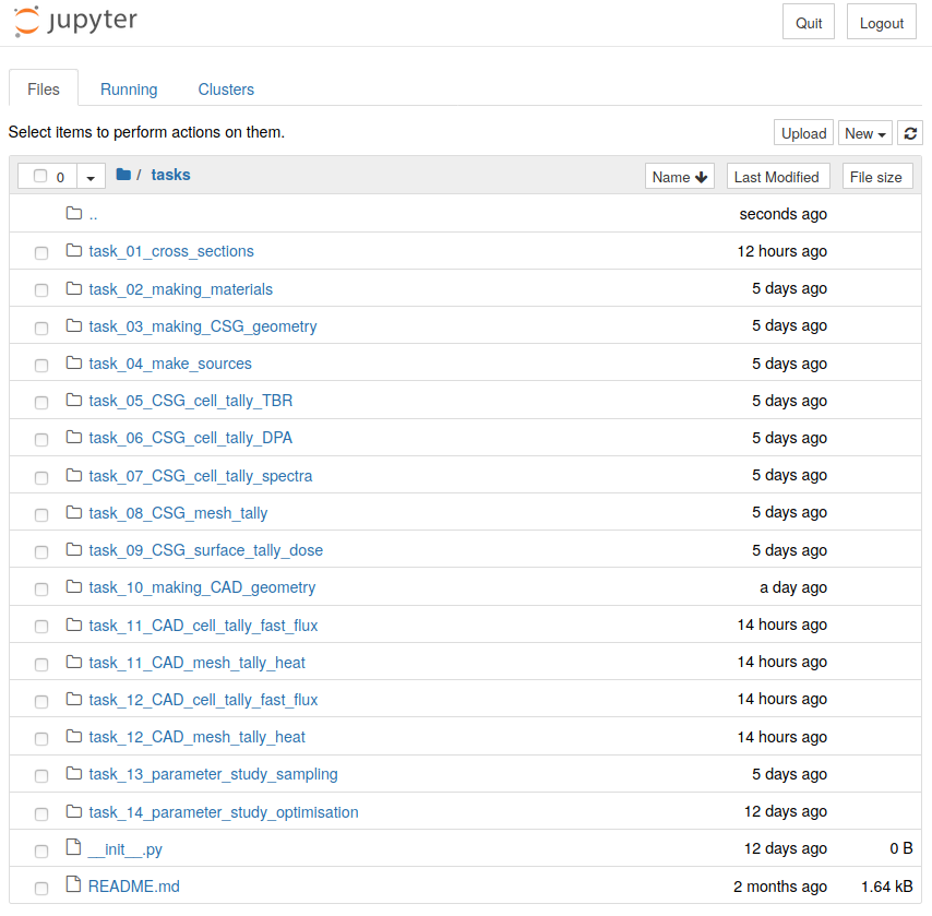
- Collection of Jupyter notebooks for each task
- Tasks have comments and instructions within the notebook
-
Outputs include
- numbers
- graphs
- images
- 3D files
- Learning outcomes from each task
Why containerisation

OpenMC popularity

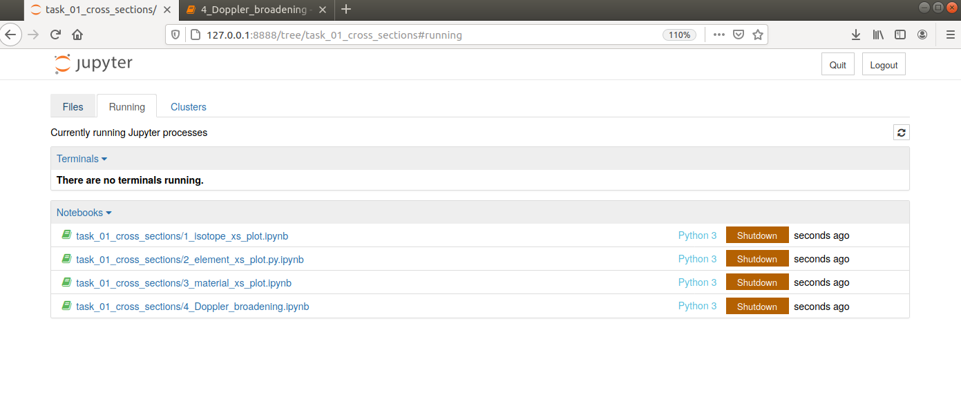
Remeber to shutdown the tasks
If your graphs are not showing it could be due to limited memory.
Switch to the Running tab
Introduction to the workshop
14:10
Introduction
Task 1 - Cross sections - parts 1, 2, 3, 4
14:00
Task 2 - Materials - parts 1, 2
Task 3 - CSG geometry parts 1, 3
Break
Task 4 - Sources - parts 1, 2, 3
Task 5 - TBR - part 1
Task 6 - DPA - part 1
Task 7 - Neutron and photon spectra - part 1 and part 2
14:40
15:15
15:45
16:20
16:30
17:15
17:30
17:55
Task 8 - Mesh tallies - parts 1 and 2
Task 10 - Making CAD geometry - part 1 and 2
15:00
17:45
Break
17:00
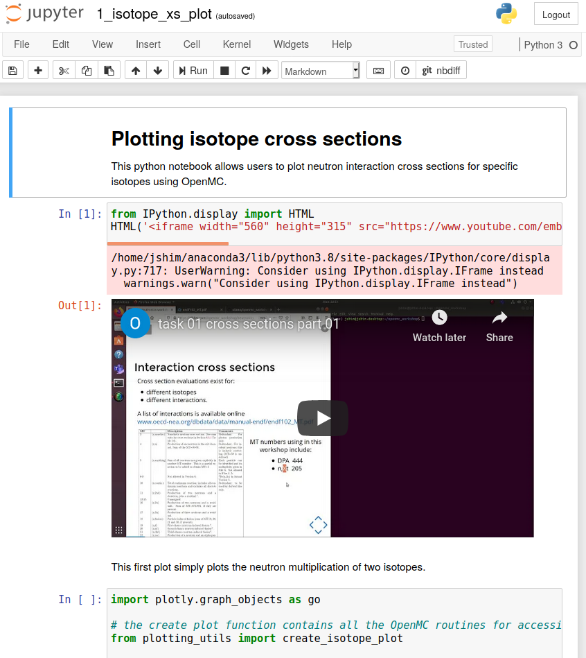
Task 1
Cross Sections
Press down to see the next slide
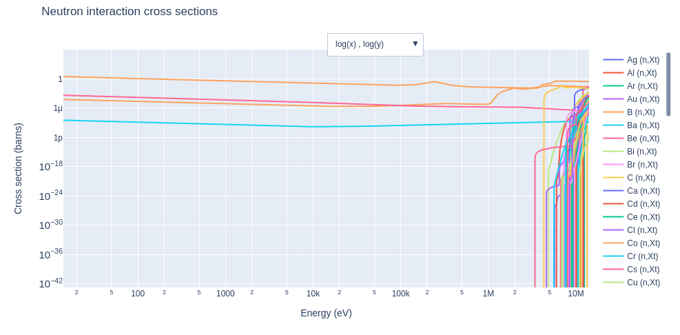
Cross section data is key to the neutronics workflow and provide us with the likelihood of a particular interaction.
Microscopic cross section
Cross sections can be measured experimentally with monoenergetic neutrons.
Probability of interaction is characterised by the microscopic cross-section (σ). It is the effective size of the nucleus.
Experimental data
Availability of experimental data varies for different reactions and different isotopes.
Typically the experimental data is then interpreted to create evaluation libraries, such as ENDF, JEFF, JENDL, CENDL.
Cross section evaluations exist for:
- different isotopes
- different interactions.
Interaction cross sections
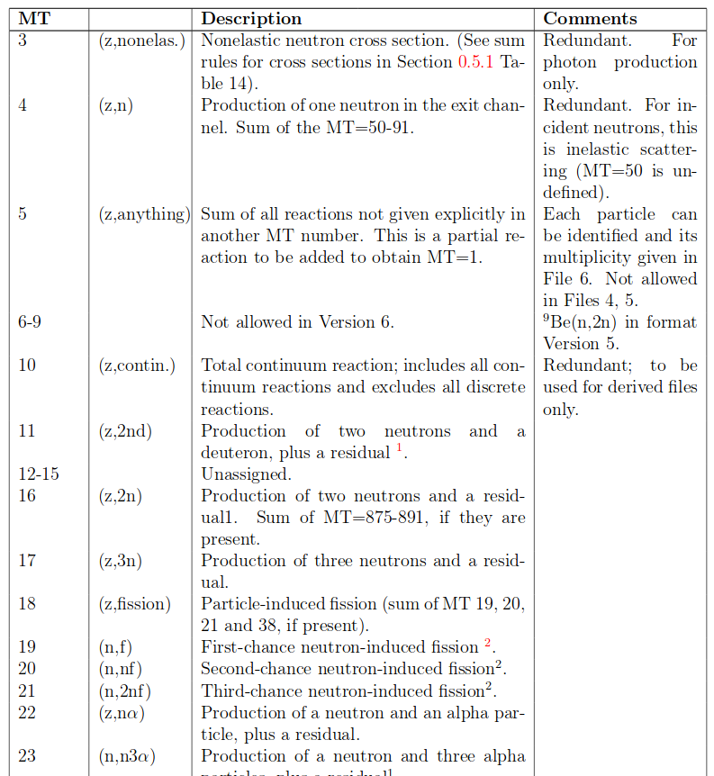
A list of interactions is available online
MT numbers using in this workshop include:
- DPA 444
- n,Xt 205
Cross section to reactions
Neutron flux (ɸ) in units of neutrons cm-2.s-1
n is number of neutrons per cm3 (neutron density)
NA is Avogadro's number (6.022e23 atoms per mole)
The atom number density (ND) is the number of atoms per cm3.
The reaction rate (RR) is the total number of neutron interaction per unit volume. Units of s-1
Macroscopic cross-section (Σ) corresponds to the total equivalent area of all the nuclei considered.
v is the neutron velocity
p is the density in gcm-3
M is the atomic weight in grams
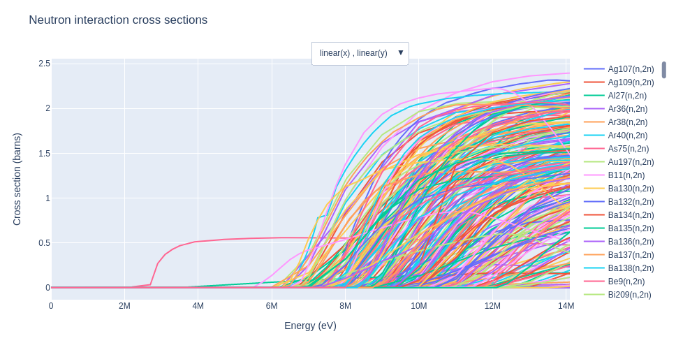
Task 1 - Cross section plotting
Isotopes

Task 1 - Cross section plotting
Isotopes
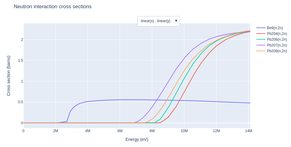
Task 1 - Cross section plotting
Isotopes
Task 1 - Cross section plotting
Elements
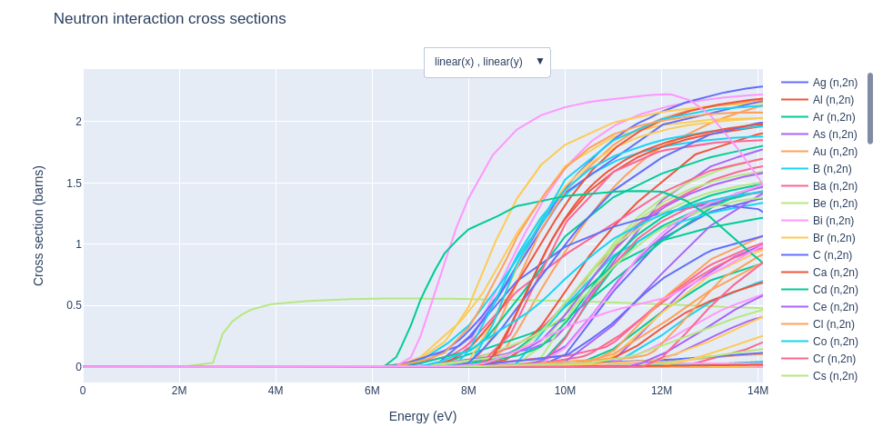
Task 1 - Cross section plotting
Elements
Task 1 - Cross section plotting
Materials

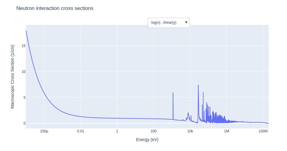
Task 1 - Cross section plotting
Materials

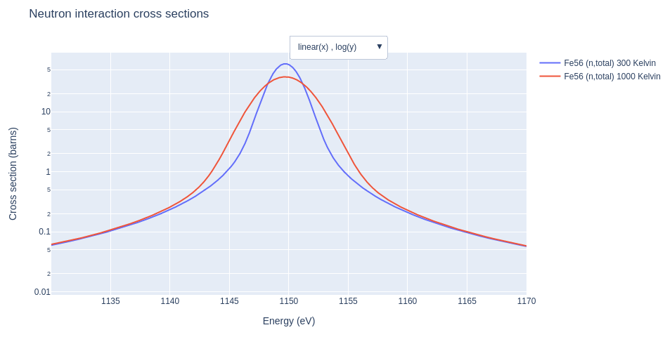
Task 1 - Cross section plotting
Doppler broadening
Task 1 - Cross section plotting
Doppler Broadening
Task 2
Materials
Press down to see the next slide
Making materials

Protons
Neutron
Neutronics codes require the isotopes and the number density.
Making materials
import openmc

mat1 = openmc.Material()
mat1.add_element('Li', 2)
mat1.add_element('O', 1)
mat1.set_density('g/cm3', 2.01)


mat2 = openmc.Material()
mat2.add_nuclide('Li6', 0.0759*2)
mat2.add_nuclide('Li7', 0.9241*2)
mat2.add_nuclide('O16', 0.9976206)
mat2.add_nuclide('O17', 0.000379)
mat2.add_nuclide('O18', 0.0020004)
mat2.set_density('g/cm3', 2.01)
Simple material construction from elements or from isotopes.
Enriching materials
Simple material construction with lithium 6 enrichment
import openmc

mat1 = openmc.Material()
mat1.add_element('Li', 2,
                 enrichment_target='Li6',
                 enrichment=60)
mat1.add_element('O', 1)
mat1.set_density('g/cm3', 2.01)


mat2 = openmc.Material()
mat2.add_nuclide('Li6', 0.6*2)
mat2.add_nuclide('Li7', 0.4*2)
mat2.add_nuclide('O16', 0.9976206)
mat2.add_nuclide('O17', 0.000379)
mat2.add_nuclide('O18', 0.0020004)
mat2.set_density('g/cm3', 2.01)
Enriching materials
import openmc

mat1 = openmc.Material()
mat1.add_elements_from_formula('Li2O',
    enrichment_target='Li6',
    enrichment=60)
mat1.set_density('g/cm3', 2.01)
Simple material construction from formula with enrichment.
Making fusion relevant materials
import openmc

mat1 = openmc.Material()
mat1.add_nuclide('Fe56', 0.8149682034000001)
mat1.add_nuclide('Fe57', 0.0188211699)
mat1.add_nuclide('Fe58', 0.0025047522000000003)
mat1.add_nuclide('Fe54', 0.05191587450000001)
mat1.add_nuclide('B10', 1.982e-06)
mat1.add_nuclide('B11', 8.018e-06)
mat1.add_nuclide('C12', 0.0010383680999999998)
mat1.add_nuclide('C13', 1.1631899999999998e-05)
mat1.add_nuclide('N15', 1.4652000000000002e-06)
mat1.add_nuclide('N14', 0.00039853480000000003)
mat1.add_nuclide('O16', 9.976206000000001e-06)
mat1.add_nuclide('O18', 2.0003999999999998e-08)
mat1.add_nuclide('O17', 3.79e-09)
mat1.add_nuclide('Al27', 4e-05)
mat1.add_nuclide('Si29', 1.2176216e-05)
mat1.add_nuclide('Si28', 0.000239797168)
mat1.add_nuclide('Si30', 8.026615999999999e-06)
mat1.add_nuclide('P31', 2e-05)
mat1.add_nuclide('S33', 2.2460700000000002e-07)
mat1.add_nuclide('S32', 2.8512222e-05)
mat1.add_nuclide('S36', 4.374e-09)
mat1.add_nuclide('S34', 1.258797e-06)
mat1.add_nuclide('Ti46', 8.250000000000001e-07)
mat1.add_nuclide('Ti49', 5.410000000000001e-07)
mat1.add_nuclide('Ti50', 5.180000000000001e-07)
mat1.add_nuclide('Ti48', 7.372e-06)
mat1.add_nuclide('Ti47', 7.44e-07)
mat1.add_nuclide('V50', 5e-06)
mat1.add_nuclide('V51', 0.0019950000000000002)
mat1.add_nuclide('Cr53', 0.0085509)
mat1.add_nuclide('Cr50', 0.0039105)
mat1.add_nuclide('Cr52', 0.0754101)
mat1.add_nuclide('Cr54', 0.0021285)
mat1.add_nuclide('Mn55', 0.0055)
mat1.add_nuclide('Co59', 5e-05)
mat1.add_nuclide('Ni60', 2.62231e-05)
mat1.add_nuclide('Ni61', 1.1399e-06)
mat1.add_nuclide('Ni58', 6.80769e-05)
mat1.add_nuclide('Ni64', 9.256000000000001e-07)
mat1.add_nuclide('Ni62', 3.6345000000000005e-06)
mat1.add_nuclide('Cu63', 2.0745000000000002e-05)
mat1.add_nuclide('Cu65', 9.255e-06)
mat1.add_nuclide('Nb93', 5e-05)
mat1.add_nuclide('Mo95', 4.7619e-06)
mat1.add_nuclide('Mo96', 5.0018999999999995e-06)
mat1.add_nuclide('Mo97', 2.8746e-06)
mat1.add_nuclide('Mo94', 2.7560999999999998e-06)
mat1.add_nuclide('Mo92', 4.3947000000000005e-06)
mat1.add_nuclide('Mo98', 7.2876e-06)
mat1.add_nuclide('Mo100', 2.9232000000000002e-06)
mat1.add_nuclide('Ta180', 1.4412e-07)
mat1.add_nuclide('Ta181', 0.0011998558799999998)
mat1.add_nuclide('W183', 0.0015741)
mat1.add_nuclide('W184', 0.0033704)
mat1.add_nuclide('W186', 0.0031273)
mat1.add_nuclide('W180', 1.3199999999999997e-05)
mat1.add_nuclide('W182', 0.002915)
mat1.set_density('g/cm3', 2.01)
There are a large number of isotopes in a material
Making fusion relevant materials
import neutronics_material_maker as nmm

ref_mat = nmm.Material('eurofer')
mat1 = ref_mat.openmc_material
There is an app for that
Open-source

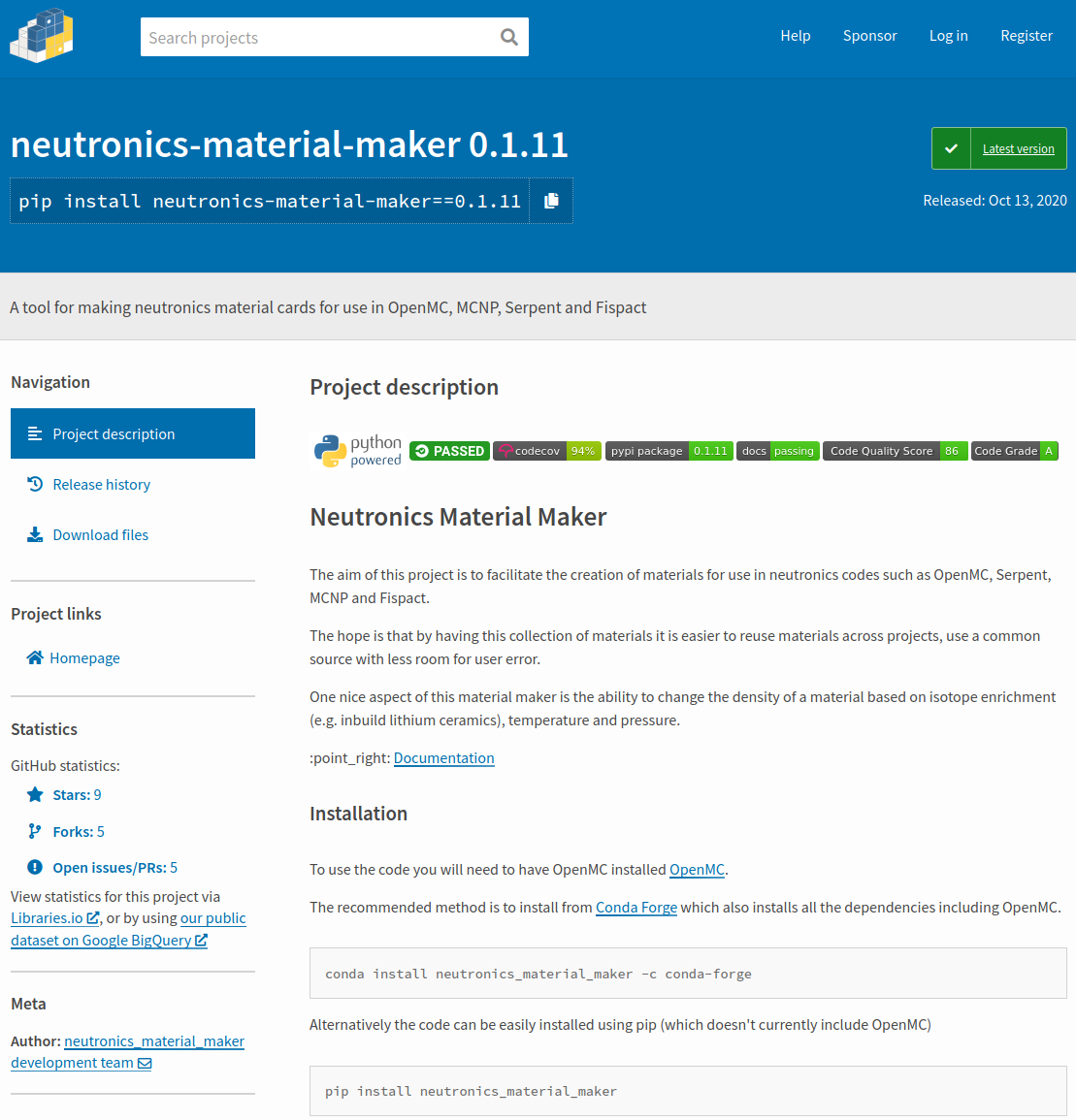
Pip install
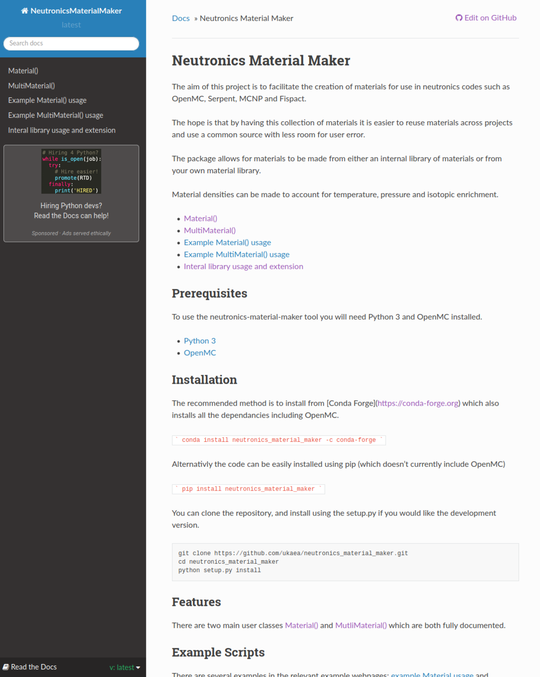
Documented
Density with temperature

Materials used in fusion reactors such as water, FLiBe, lithium lead change density with temperature.
The NeutronicsMaterialMaker finds the density automatically
Density with pressure

Materials used in fusion reactors such as helium and CO2 change density with pressure.
The NeutronicsMaterialMaker finds the density automatically
Density with Li6 enrichment

Materials used in fusion reactors such as Li4SiO4 and Li2SiO3.
The NeutronicsMaterialMaker finds the density automatically
Task 3
CSG geometry
Press down to see the next slide
Making geometry
import openmc

surface_sphere = openmc.Sphere(r=10.0)
region_inside_sphere = -surface_sphere
cell_sphere = openmc.Cell(region=region_inside_sphere)

cell_sphere.fill = steel
import openmc
surf_sphere1 = openmc.Sphere(r=10.0)
surf_sphere2 = openmc.Sphere(r=20.0)
between_spheres = +surf_sphere1 & -surf_sphere2
cell_between = openmc.Cell(region= between_spheres)
cell_between.fill = steelEnd of the universe
import openmc

surface_sphere = openmc.Sphere(r=10.0)
region_inside_sphere = -surface_sphere
cell_sphere = openmc.Cell(region=region_inside_sphere)
import openmc

surf_sphere = openmc.Sphere(r=10.0, boundary_type="vacuum")
between_spheres = -surf_sphere
cell_between = openmc.Cell(region= between_spheres)
The outer most surface must be identified using the boundary_type keyword
Particles crossing this surface are no longer tracked by the code and are terminated.
Making geometry
Making surfaces
surface_xp = openmc.XPlane(x0=0)
surface_yp = openmc.YPlane(y0=0)
surface_zp = openmc.ZPlane(z0=0)
surface_p = openmc.Plane(A=1.0, B=0.0, C=0.0, D=0.0)
surface_xcy = openmc.XCylinder(y0=0.0, z0=0.0, R=1.0)
surface_ycy = openmc.YCylinder(x0=0.0, z0=0.0, R=1.0)
surface_zcy = openmc.ZCylinder(x0=0.0, z0=0.0, R=1.0)
surface_s = openmc.Sphere(x0=0.0, y0=0.0, z0=0.0, R=1.0)
surface_xco = openmc.XCone(x0=0.0, y0=0.0, z0=0.0, R2=1.0)
surface_yco = openmc.YCone(x0=0.0, y0=0.0, z0=0.0, R2=1.0)
surface_zco = openmc.ZCone( x0=0.0, y0=0.0, z0=0.0, R2=1.0)
surface_quad = openmc.Quadric(a=0.0, b=0.0, c=0.0, d=0.0, e=0.0, f=0.0, g=0.0, h=0.0, j=0.0, k=0.0)
OpenMC makes use of constructive solid geometry (CSG)
CAD geometry is also supported via DAGMC
✅
✅
✅
Making geometry
Making volumes
| (union)
import openmc

surf_sphere = openmc.Sphere(r=20.0)

surf_cy = openmc.ZCylinder(r=5)
surf_up_zp = openmc.ZPlane(z0=30)
surf_low_zp = openmc.ZPlane(z0=-30)

region_sph = -surf_sphere
region_cy = (-surf_cy & -surf_up_zp & +surf_low_zp)

cell = openmc.Cell(region = region_sph | region_cy)

cell_sphere.fill = steel
|
=
Making geometry
Making volumes
~ (complement)
import openmc

surf_sphere1 = openmc.Sphere(r=20.0)

surf_cy = openmc.ZCylinder(r=5)
surf_up_zp = openmc.ZPlane(z0=30)
surf_low_zp = openmc.ZPlane(z0=-30)

region_sph = -surf_sphere2
region_cy = (-surf_cy & -surf_up_zp & +surf_low_zp)

cell = openmc.Cell(region = region_sph & ~region_cy)

cell_sphere.fill = steel
~
=
Making geometry
Making volumes
& (intersection)
import openmc

surf_sphere1 = openmc.Sphere(r=20.0)

surf_cy = openmc.ZCylinder(r=5)
surf_up_zp = openmc.ZPlane(z0=30)
surf_low_zp = openmc.ZPlane(z0=-30)

region_sph = -surf_sphere2
region_cy = (-surf_cy & -surf_up_zp & +surf_low_zp)

cell = openmc.Cell(region = region_cy & region_sph)

cell_sphere.fill = steel
&
=
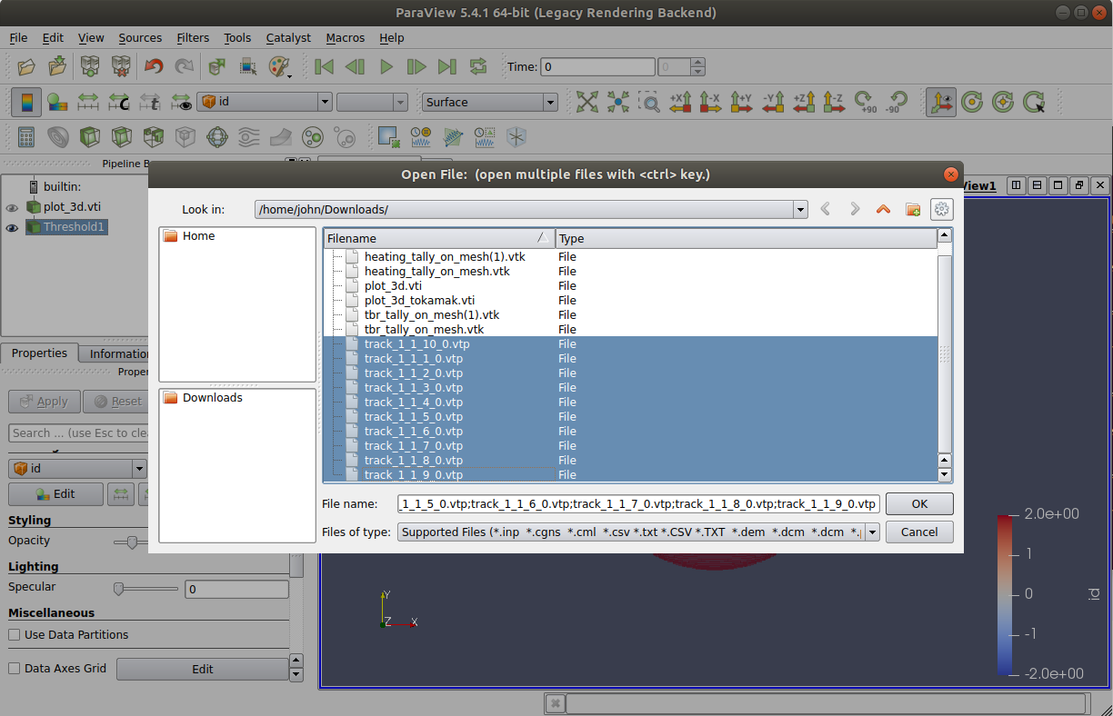
Building and visualizing CSG geometry


Building and visualizing CSG geometry

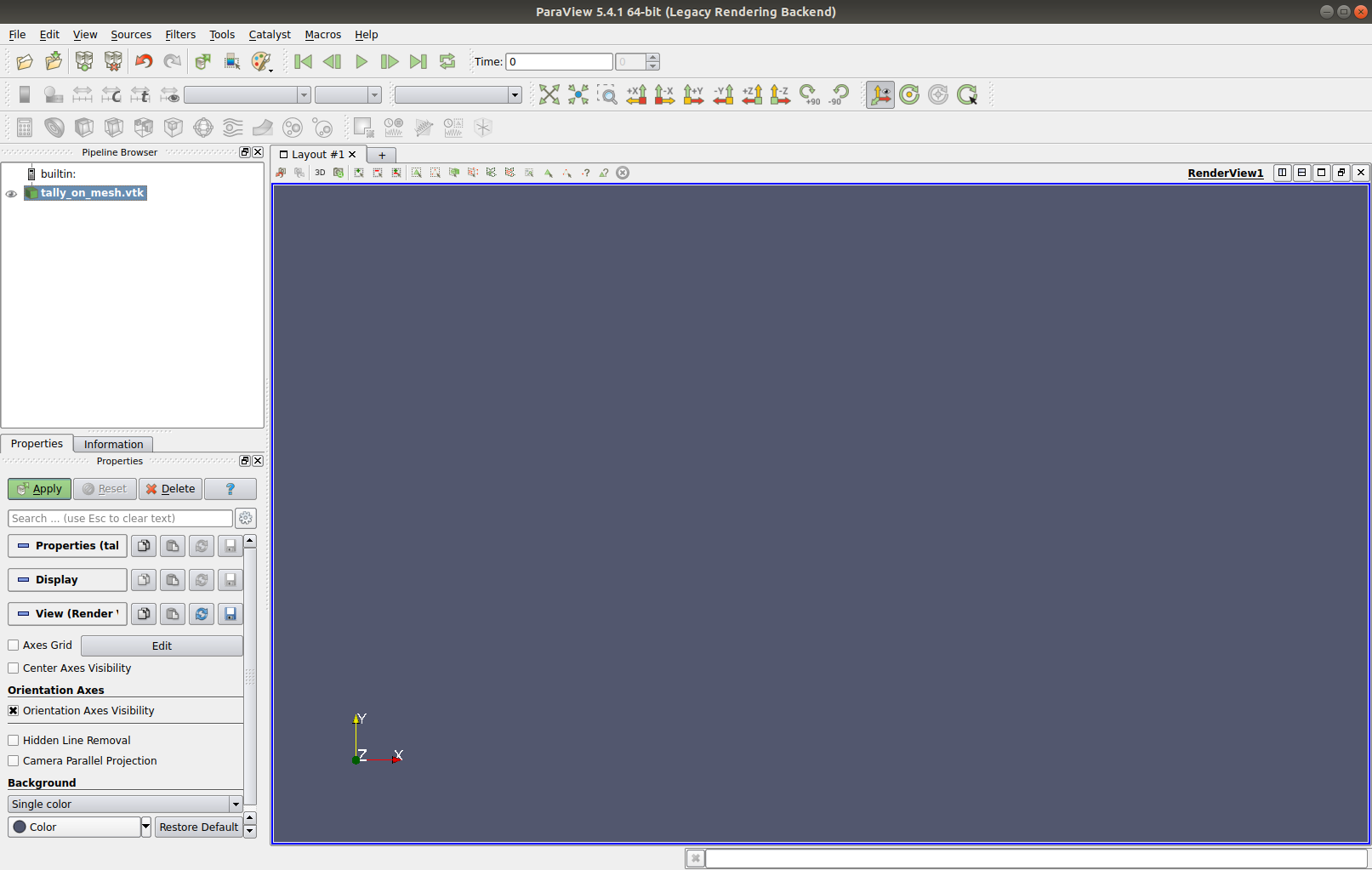
Visualizing CSG geometry in 3D


hints

Open file and click 'Apply'
to initiate geometry viewing
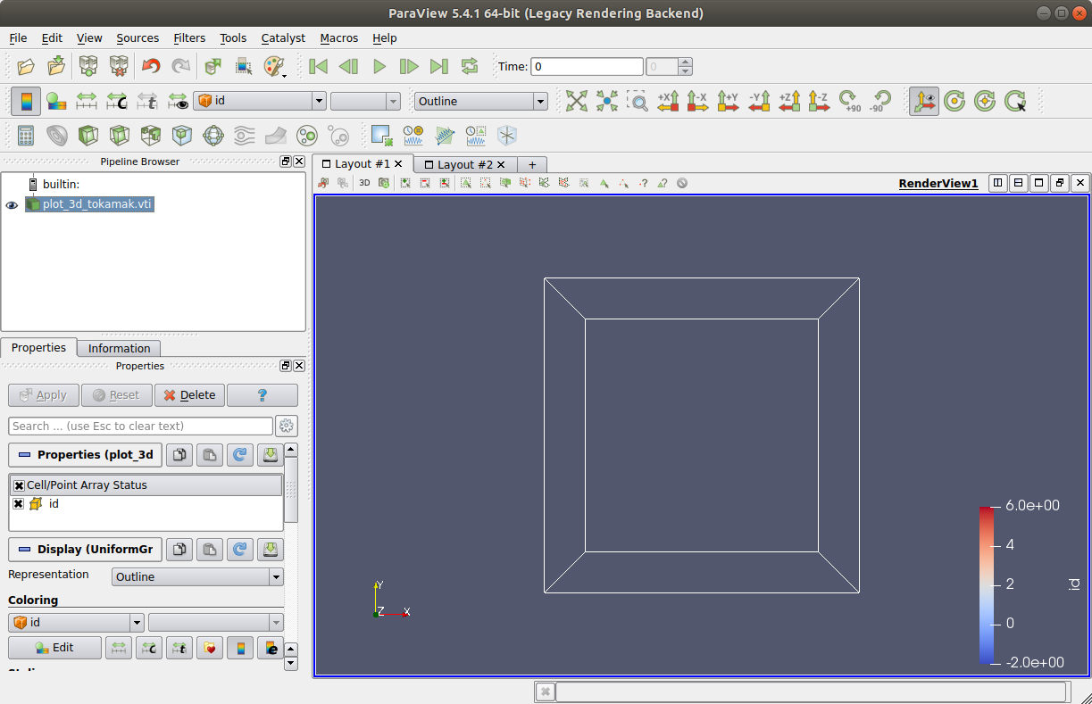
hints
Use eyeball icon to toggle between displaying and hiding geometry

hints
Specify geometry to be coloured
with respect to cell ID
hints
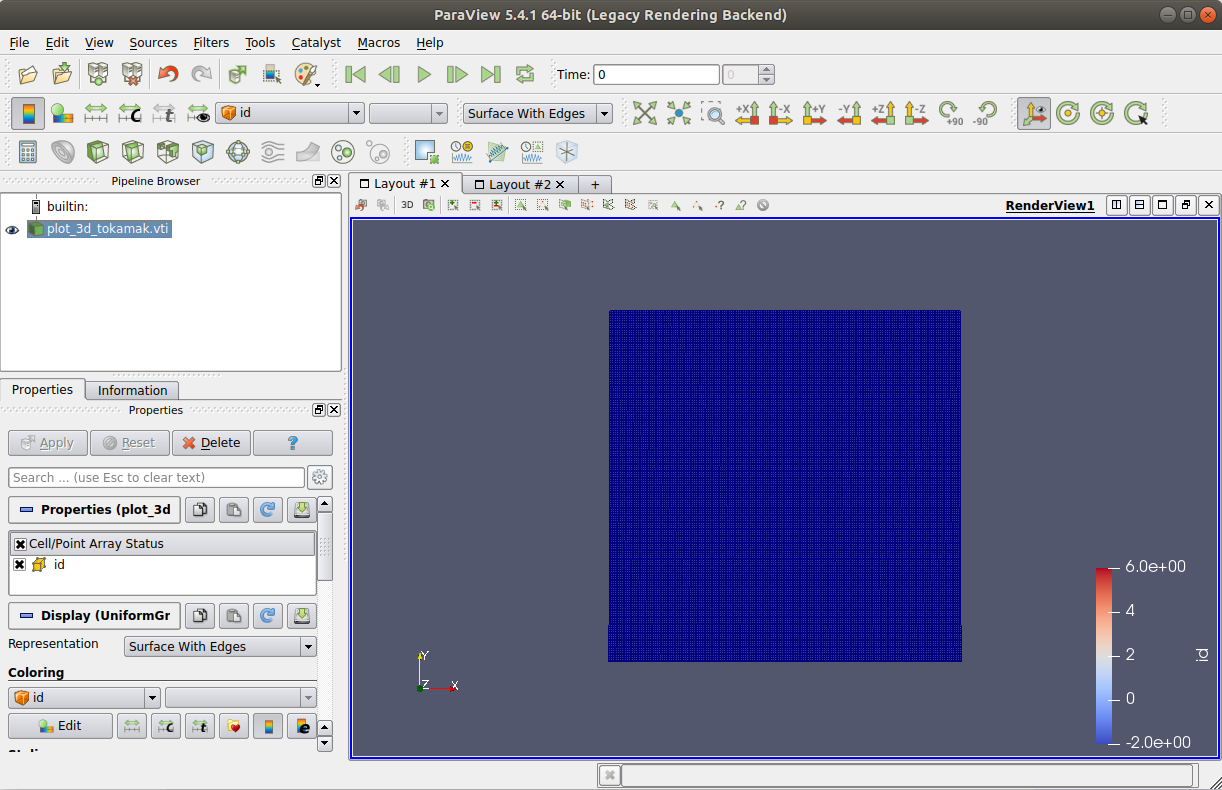
Display geometry
surfaces

hints
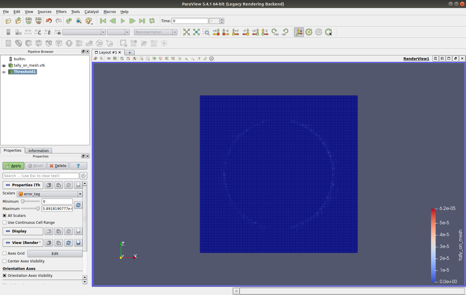
Perform a threshold to isolate the geometry of interest (paraview automatically shows all geometry cells specified in OpenMC, including vacuum cells)
hints
Change threshold limits to isolate the geometry cells of interest (click 'Apply' to perform the threshold)
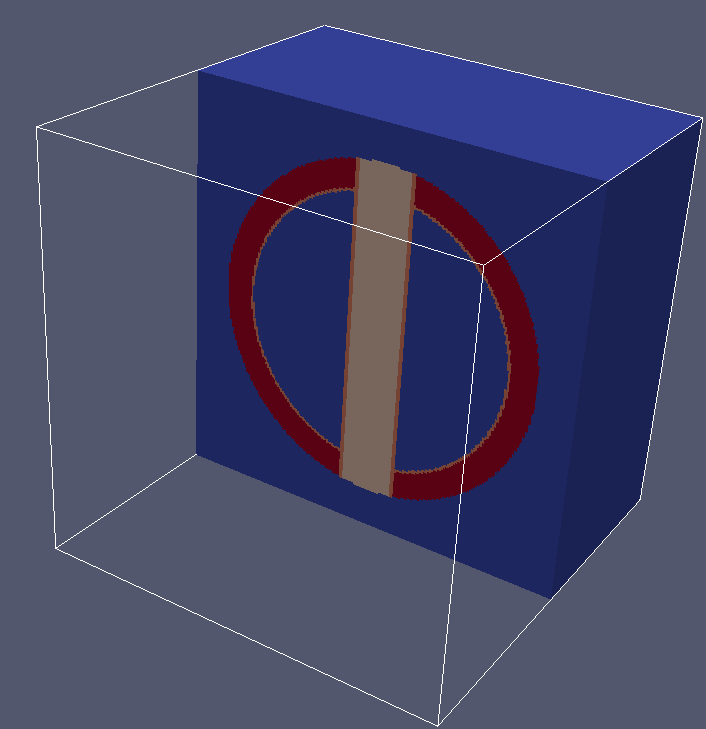
hints
Threshold function has removed the vacuum cells, allowing the geometry
to be viewed

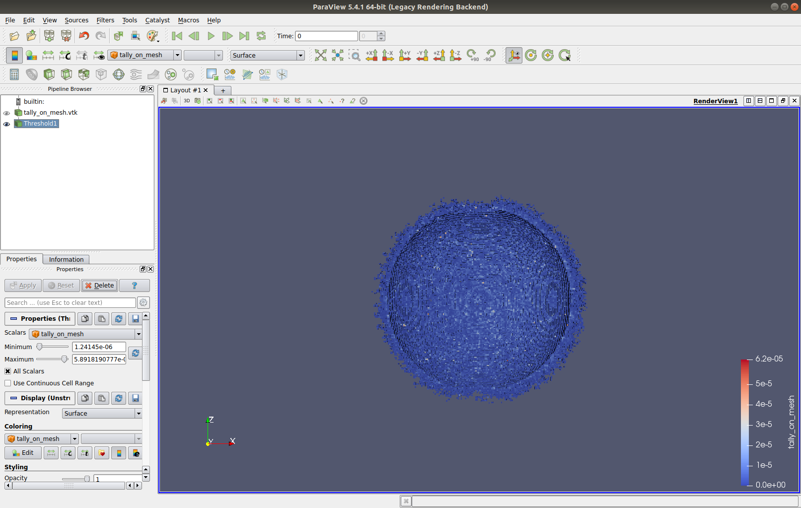
hints
Shell can be clipped to view its structure more clearly

hints
Clipping plane can be
changed using these buttons

hints
Apply the clip

hints
View can be rotated
Task 4
Sources
Press down to see the next slide
Making neutron sources
Point source birth locations

import openmc

source = openmc.Source()
source.space = openmc.stats.Point((0, 0, 0))
Making neutron sources
Point source birth directions

import openmc

source = openmc.Source()
source.angle = openmc.stats.Isotropic()
Making neutron sources
14 MeV monoenergetic

import openmc

source = openmc.Source()

# sets the location of the source to x=0 y=0 z=0
source.space = openmc.stats.Point((0, 0, 0))

# sets the direction to isotropic
source.angle = openmc.stats.Isotropic()

# sets the energy distribution to 100% 14MeV neutrons
source.energy = openmc.stats.Discrete([14e6], [1])
Making neutron sources
Watt distribution

import openmc

source = openmc.Source()
source.space = openmc.stats.Point((0, 0, 0))
source.angle = openmc.stats.Isotropic()

# Documentation on the Watt distribution is here
# https://docs.openmc.org/en/stable/pythonapi/generated/openmc.data.WattEnergy.html
source.energy = openmc.stats.Watt(a=988000.0, b=2.249e-06)
Energy distribution
Deuterium (D)
Tritium (T)
Helium 4
3.5MeV
1/5 of the energy
Neutron
14.1MeV
4/5 of the energy
Helium 5
17.6MeV
Making neutron sources
Muir distribution

import openmc

source = openmc.Source()
source.space = openmc.stats.Point((0, 0, 0))
source.angle = openmc.stats.Isotropic()

# Documentation on the Muir distribution is here
# https://docs.openmc.org/en/stable/pythonapi/generated/openmc.stats.Muir.html
source.energy = openmc.stats.Muir(
  e0=14080000.0,
  m_rat=5.0,
  kt=20000.0
)
MCF and ICF
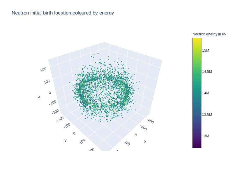
Making neutron sources
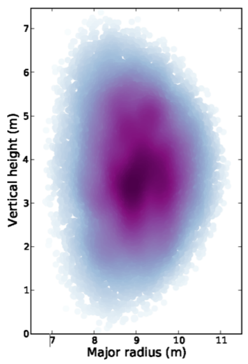
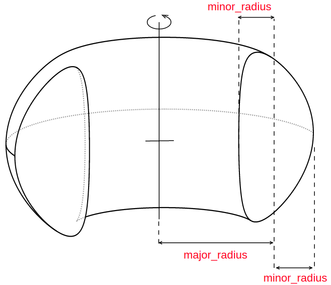
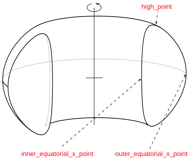
Plasma source birth locations

import openmc

from parametric_plasma_source

import PlasmaSourcemy_plasma = PlasmaSource(
    elongation=1.557,
    ion_density_origin=1.09e20,
    ion_density_peaking_factor=1,
    ion_density_pedestal=1.09e20,
    ion_density_separatrix=3e19,
    ion_temperature_origin=45.9,
    ion_temperature_peaking_factor=8.06,
    ion_temperature_pedestal=6.09,
    ion_temperature_separatrix=0.1,
    major_radius=9.06,
    minor_radius=2.92,
    pedestal_radius=0.8 * 2.92,
    plasma_id=1,
    shafranov_shift=0.44789,
    triangularity=0.270,
    ion_temperature_beta=6
)
Making neutron sources
Plasma source birth directions

import openmc

from parametric_plasma_source

import PlasmaSourcemy_plasma = PlasmaSource(
    elongation=1.557,
    ion_density_origin=1.09e20,
    ion_density_peaking_factor=1,
    ion_density_pedestal=1.09e20,
    ion_density_separatrix=3e19,
    ion_temperature_origin=45.9,
    ion_temperature_peaking_factor=8.06,
    ion_temperature_pedestal=6.09,
    ion_temperature_separatrix=0.1,
    major_radius=9.06,
    minor_radius=2.92,
    pedestal_radius=0.8 * 2.92,
    plasma_id=1,
    shafranov_shift=0.44789,
    triangularity=0.270,
    ion_temperature_beta=6
)
Making neutron sources
Photon source energy spectrum
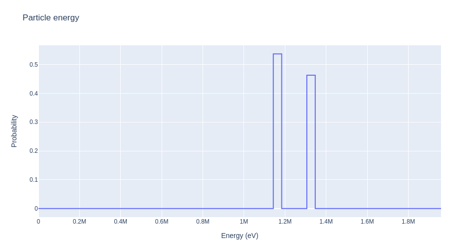
import openmc

# initialises a new source object
source = openmc.Source()

# sets the location of the source to x=0 y=0 z=0
source.space = openmc.stats.Point((0, 0, 0))

# sets the direction to isotropic
source.angle = openmc.stats.Isotropic()

# sets the energy distribution to
# 50% 1.1MeV photons and 50% 1.3MeV photons
source.energy = openmc.stats.Discrete(
  [1.1732e6,1.3325e6],
  [0.5, 0.5]
)

# change particle type as the default is neutron
source.particle = 'photon'
hints

Open and threshold geometry
as shown in Task 3
hints

Reduce opacity of threshold
geometry to increase its transparency -
this allows neutron tracks to be seen
more easily
hints
Open .vtp track files
hints
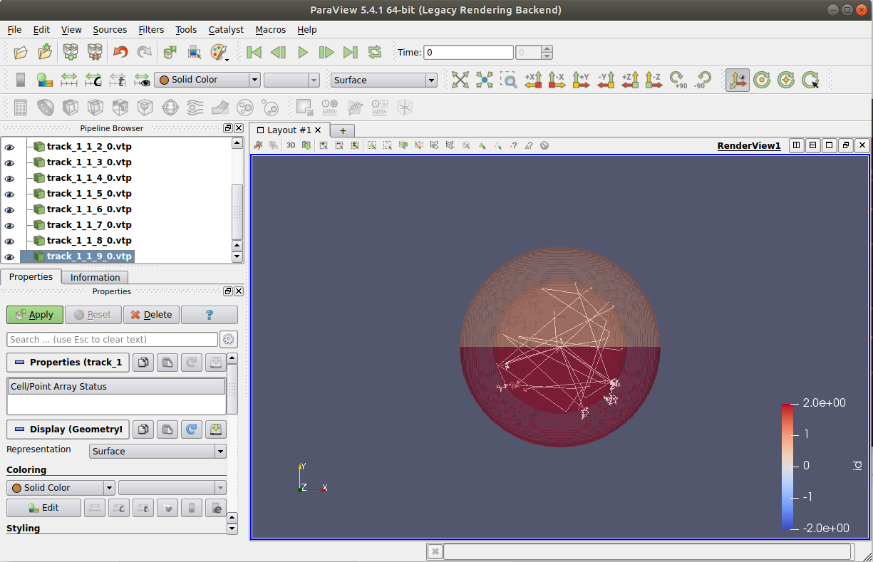
Toggle visibility of each .vtp
file to view neutron tracks
Task 5
CSG cell tally - TBR
Press down to see the next slide
Task 5
CSG tally - TBR
TBR parameter study

Task 6
CSG cell tally - DPA
Press down to see the next slide
Task 6
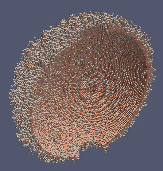
Displacement
Finding the neutron damage

IAEA Issues Crowdsourcing Challenge for Materials for Fusion Technology
A visualization of the cascade of collisions leading to damage in a crystalline material. (Photo: A. Sand/University of Helsinki)
Stochastic volume calculation

Task 7
CSG cell & surface tally - spectra
Press down to see the next slide
Neutron interactions
Material 1
Material 2
Neutron birth
(n,n')
(n,f)
(n,n')
(γ,γ')
(n,nγ')
(n,pn')
(n,f)
(n,2n)
(n,α)
(n,γ)
Neutron
Electron
Gamma
Alpha
Proton
Types of scattering
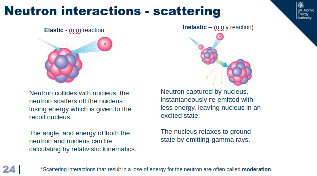
Neutron collides with the nucleus, the neutron scatters of the nucleus losing energy which is given to the recoil nucleus.
The angle and energy of both the neutron and he nucleus can be calculated by relativistic kinematics
Neutron capture by nucleus instantaneously re-emitted with less energy, leaving the nucleus in an excited state.
The nucleus relaxes to ground state by emitting gamma rays.
Angle
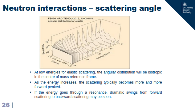
- At low energies the angular distribution is often isotropic in the center of mass reference frame.
- As the energy increases the scattering typically becomes more and more forward peaked.
- If the energy goes through a resonance, dramatic swings from forwards scattering to backwards may be seen.
Image from tendl.web.psi.ch
Path length
Path length = 1 / Macroscopic cross section
Shorter path length for lower neutron energy
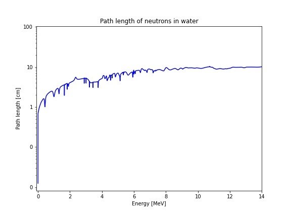
Path length
- A 14MeV neutron will lose energy via scattering interactions.
- The average path length between scattering interactions decreases.
- Once thermalised the there is equal chance of energy lose or energy gain via collision.
- Path length at thermal energy is more constant
Equations
The average logarithmic energy decrement (or loss) per collision (ξ) is related to the atomic mass (A) of the nucleus
| Hydrogen | Deuterium | Beryllium | Carbon | Uranium | |
|---|---|---|---|---|---|
| Mass of nucleus | 1 | 2 | 9 | 12 | 238 |
| Energy decrement | 1 | 0.7261 | 0.2078 | 0.1589 | 0.0084 |
Collisions
| Hydrogen | Deuterium | Beryllium | Carbon | Uranium | |
|---|---|---|---|---|---|
| Number of collisions to thermalize | 20 | 25 |
85 | 115 | 2172 |
The average number of collisions requried to reduce the energy of the neutron from Eo to E
*where a thermal neutron energy = 0.025eV
Moderating power
We should account for the likelihood of scattering.
| Water | Heavy water | Beryllium | Carbon | Polyethylene | |
|---|---|---|---|---|---|
| Moderating power | 1.28 | 0.18 | 0.16 | 0.064 | 3.26 |
The number density of the nucleus (ND) and the microscopic cross section (σ) combine to produce the macroscopic scattering cross section (Σ)
Moderating ratio
| Water | Heavy water | Beryllium | Carbon | Polyethylene | |
|---|---|---|---|---|---|
| Moderating ratio | 58 | 2100 | 130 | 200 | 122 |
The probability of being absorbed is also important.
The Moderating ratio is a relative measure of a moderator to scatter neutrons without absorbing them.
Finding the neutron spectra
Neutron flux spectrum - Cell

Finding the neutron
Neutron current spectra - Surfaces

Finding the photon spectra
Photon flux spectrum - Cell

Task 8
CSG mesh tally
Press down to see the next slide
CSG regular mesh tally
# only 1 cell in the Y dimension
mesh.dimension = [4, 1, 4]

# physical limits (corners) of the mesh
mesh.lower_left = [-200, -1, -200]
mesh.upper_right = [200, 1, 200]
# only 1 cell in the Y dimension
mesh.dimension = [4, 4, 4]

# physical limits (corners) of the mesh
mesh.lower_left = [-200, -200, -200]
mesh.upper_right = [200, 200, 200]
2D mesh tally


Flux
Absorption
(n,2n)
Geometry
3D mesh tally


Click 'Apply' to initiate
tally viewing
hints
Specify colouring with
respect to tally value

hints
Display tally surfaces

hints
Rotate to view
tally more clearly

hints
Perform a threshold to
isolate the mesh tally
hints
Change threshold limits to
isolate tally range of interest

hints
Apply the threshold to view
tally results
hints
Task 9
CSG surface tally - dose
Press down to see the next slide
Dose
Effective dose coefficients

Dose
CSG cask geometry

Dose
CSG nested sphere cask geometry

Dose
CSG nested sphere cask dose

Task 10
CAD geometry
Press down to see the next slide
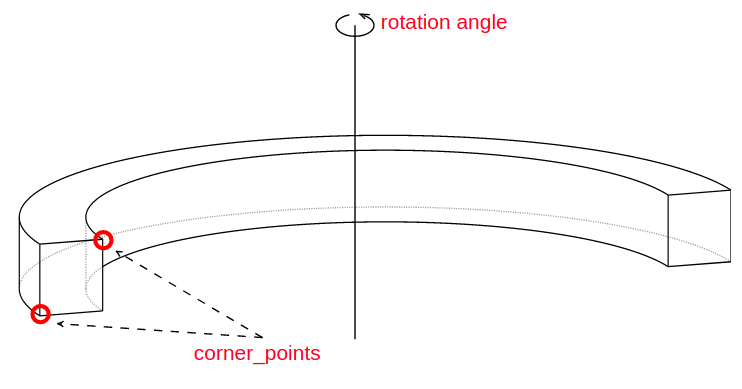
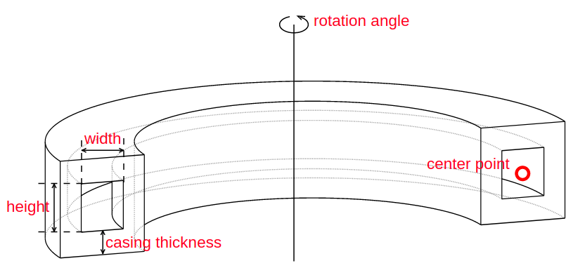
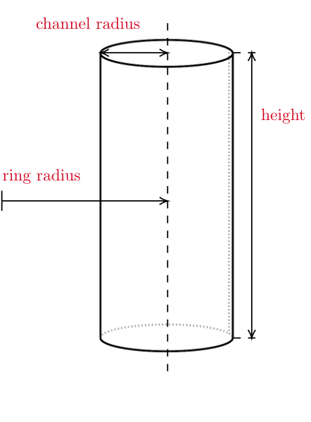
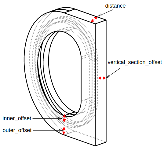
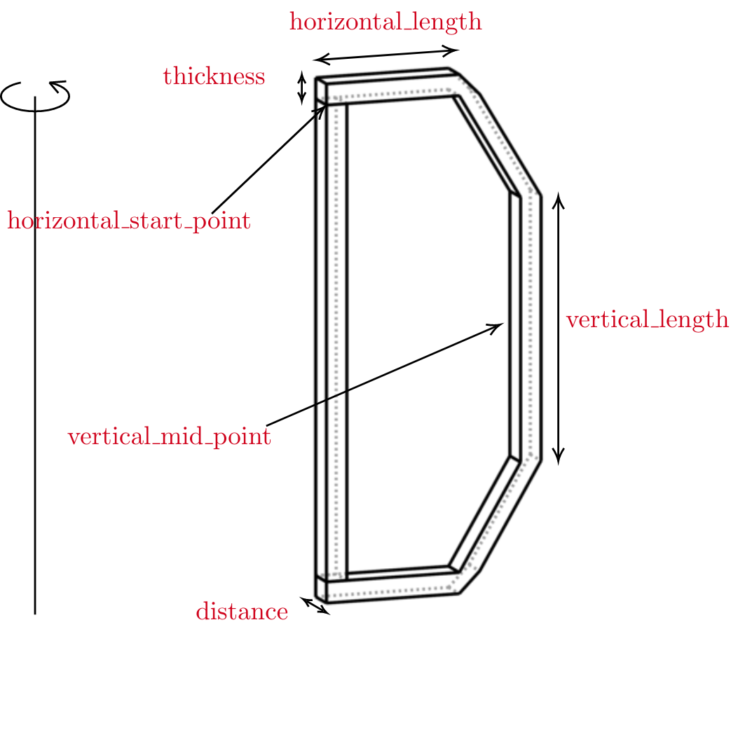
Making CAD shapes

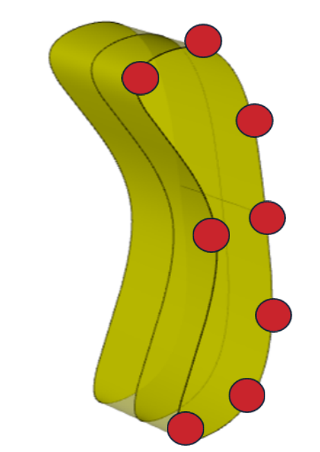
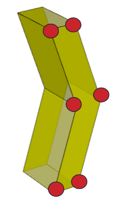
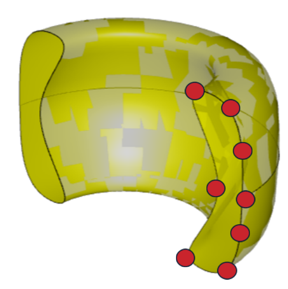
3D CAD geometry can be made by linking coordinates together with edges.
Edges can be straight, lines, splines, circles etc.
The resulting face can then be rotated, extrude of swept to make a volume.
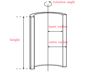
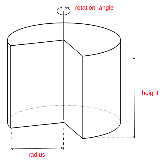
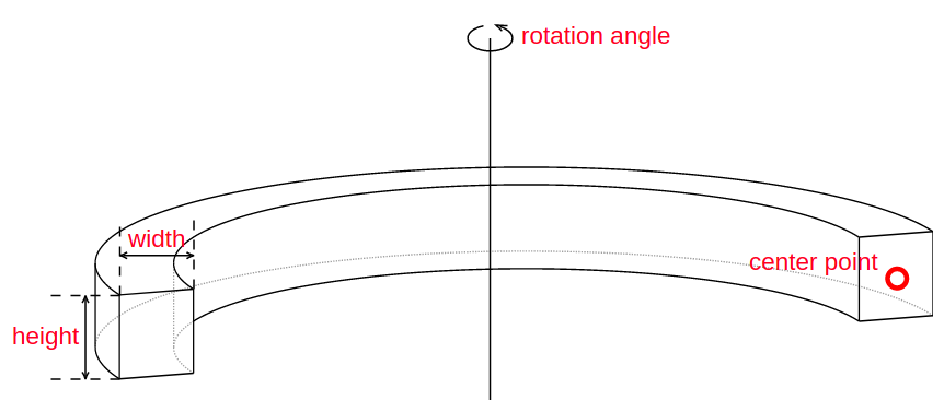
RotateStraightShape
RotateSplineShape
ExtrudeSplineShape
ExtrudeStraightShape
The volume can then undergo Boolean opperations such as cut, intersected or unioned
Making CAD components
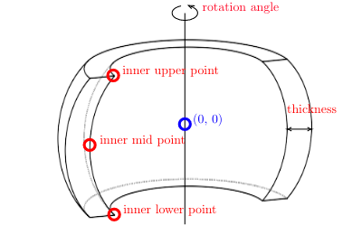
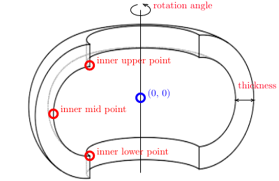
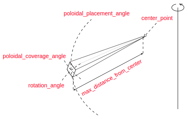

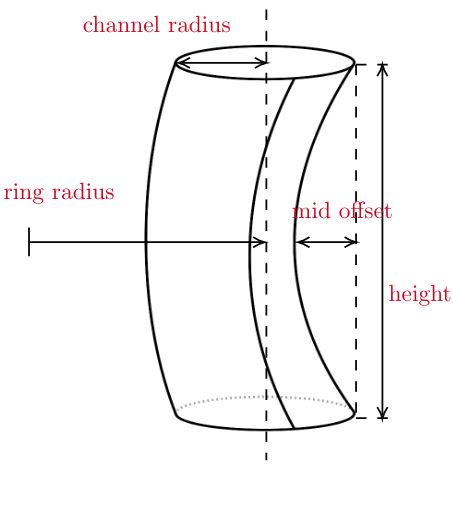
Finding the coordinates can be performed automatically by using a component.
Component construction is driven by parameters.
Boolean operations are also available.

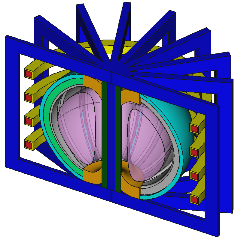
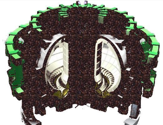
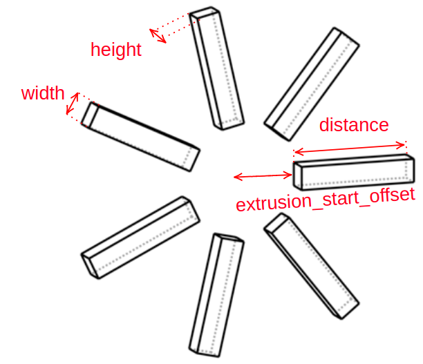
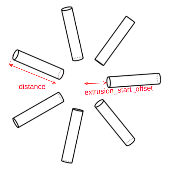
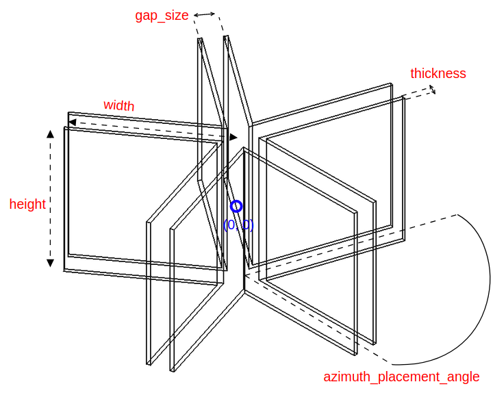
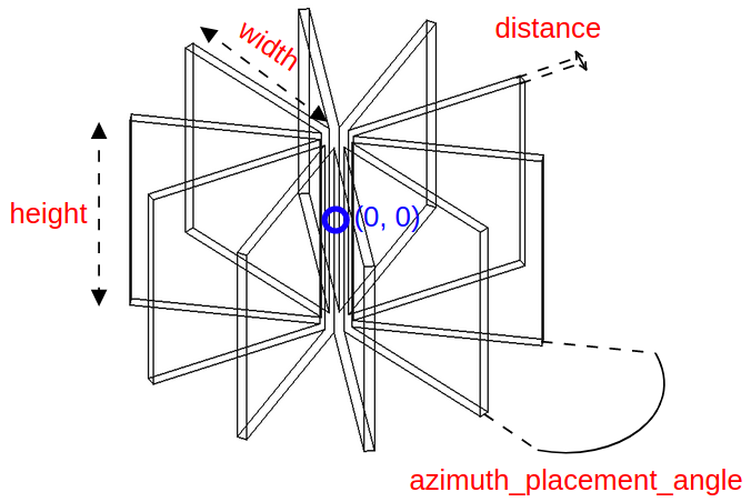
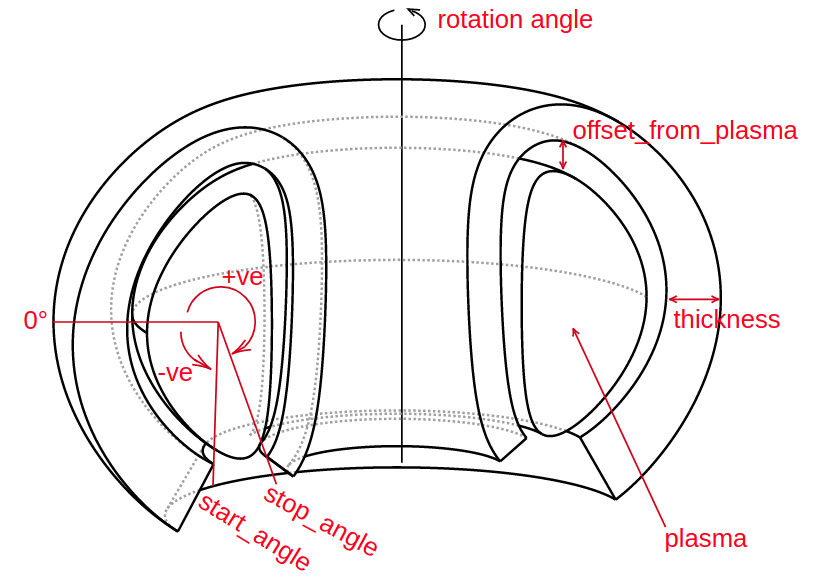
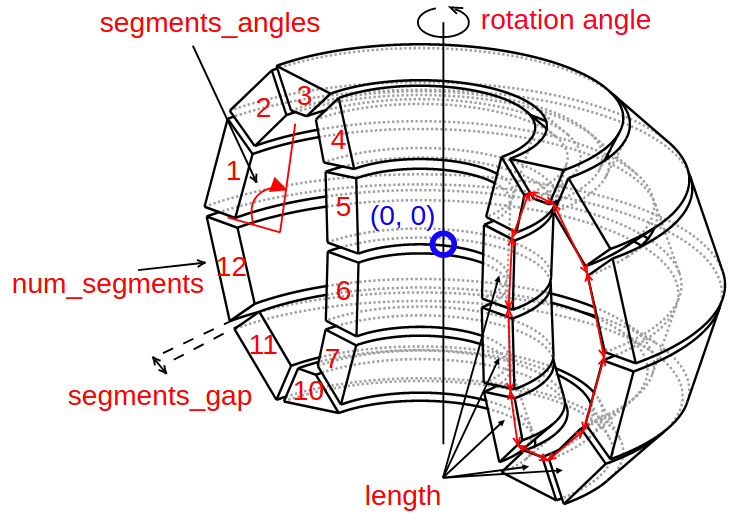
Making CAD reactors
Components and Shapes can be assembled into reactors.
The construction is parameter driven.
Shapes / components


Plasma
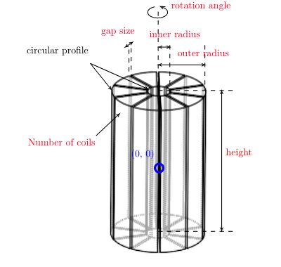
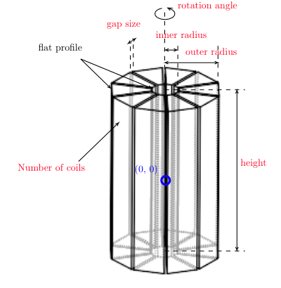
TF coils
PF coils
Blanket
Reactor object

my_reactor = paramak.Reactor([pf_1, tf, blanket, plasma])Ball reactor

Task 11
CAD - cell tally
Press down to see the next slide
Task 12
CAD - mesh tally
Press down to see the next slide
Task 13
Parametric study sampling
Press down to see the next slide
Techniques for sampling design space - Random

Techniques for sampling design space - Grid

Techniques for sampling design space - Halton

Techniques for sampling design space - Adaptive

Task 14
Parametric study optimisation
Press down to see the next slide
Optimize a breeder
blanket for tritium production
Task currently under development
Task 15
Activation
Press down to see the next slide
Task 15
Activation
Target
Nuclide
n,2n
n,g
n,p
n,pn
n,d
n,t
n,nd
n,a
n,He3
n,pd
n = neutron
g = gamma
t = tritium
p = proton
d = deuterium
He = helium
Common neutron induced reactions
Neutron number
Proton number
Task 15
Activation
Fe56
Neutron induced reactions in Fe56
Neutron number
Proton number
Fe57
Fe58
Fe59
Fe55
Fe54
Co59
Mn53
Mn54
Mn55
Mn56
Mn57
Mn58
Cr57
Cr56
Cr55
Cr54
Cr53
Cr52
Co58
Co57
Co56
Co60
Decay
Primary activation
Secondary activation
Co55
Task 15
Activation


Task 15
Irradiation Activation
Time
Number of atoms

Shut down
- New isotopes build up during irradiation
-
Radioactive isotopes decay and will eventually reach a point where decay rate is equal to activation rate.
-
Decay is more noticeable once the plasma is shutdown.
- The activity is related to the irradiation time and the nuclide half life.
- The decay process emits gamma rays leading to dose.
- The dose is dependent on the activity, the energy of the gamma and biological response.
Task 15
Activation
https://www.surveymonkey.co.uk/r/YCCSMZN