Machine Learning

Nicholas Browning

Support Vector Machines (SVM)

Kernel Methods

Kernel Ridge Regression

Bayesian Probability Theory

Bayesian Networks

Naive Bayes

Perceptrons

Neural Networks

Principle Component Analysis

Dimensionality Reduction

Learning Theory

RDF Networks

Collaborative Filtering

Regression

GA-QMML: Prediction of Molecular Properties (QM), through Genetic Algorithm (GA) Optimisation and Non-Linear Kernel Ridge Regression (ML)

Topics of Seminar Series

Ridge Regression

  • Machine Learning introduction

  • ​Types of Learning

    • ​Supervised, Semisupervised, Unsupervised, Reinforcement

  • ​ML Applications

    • ​​​Classification, Regression, Clustering, Recommender Systems, Embedding

  • Theoretical Introduction: Regression

    • Bias-Variance trade-off, Overfitting, Regularization

Today

What is Machine Learning?

“A computer program is said to learn from experience E with respect to some task T and some performance measure P, if its performance on T, as measured by P, improves with experience E.” -- Tom Mitchell, Carnegie Mellon University

Supervised

Unsupervised

Semisupervised

Reinforcement Learning

< \vec x, f(\vec x) >
<x,f(x)>< \vec x, f(\vec x) >
< \vec D >
<D>< \vec D >
< \vec x_i , f_j(\vec x_i) >
<xi,fj(xi)>< \vec x_i , f_j(\vec x_i) >
< \vec s, \vec a >
<s,a>< \vec s, \vec a >
P( s' | a, s)
P(sa,s)P( s' | a, s)
R(s, a, s')
R(s,a,s)R(s, a, s')

Types of Machine Learning

ML Applications

From data to discrete classes

Classification

Spam Filtering

Object Detection

Weather Prediction

Medical Diagnosis

?

?

?

?

?

?

?

?

Predicting numeric value

Regression

Stock Markets

Weather Prediction

Discovering structure in data

Clustering

Natural document clusters of bio-medical research

Finding what user might want

Recommender Systems

Visualising data

Embedding

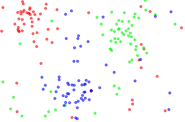
Article classification via t-Distributed Stochastic Neighbor Embedding (t-SNE)

Word classification via t-SNE

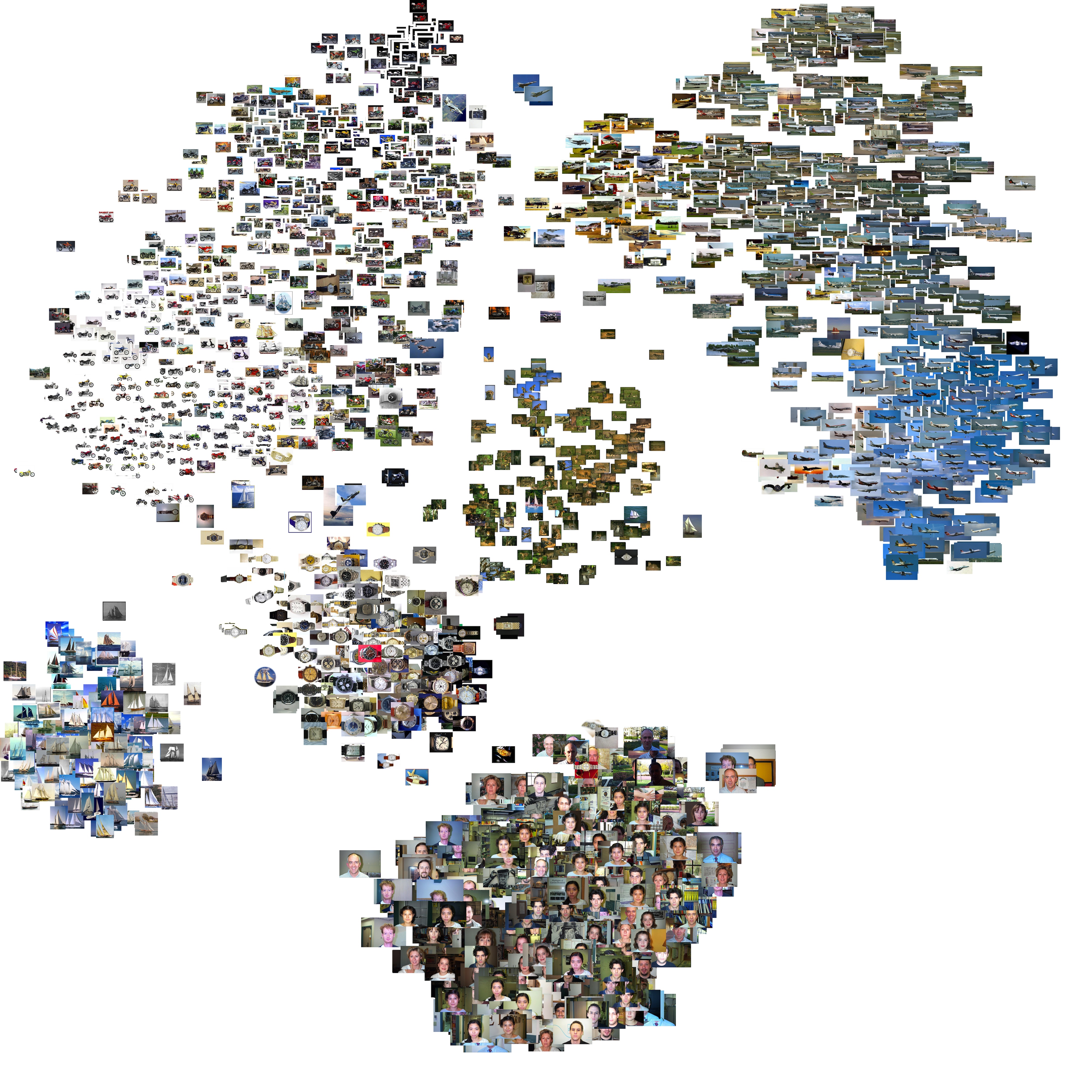
Picture classification via t-SNE

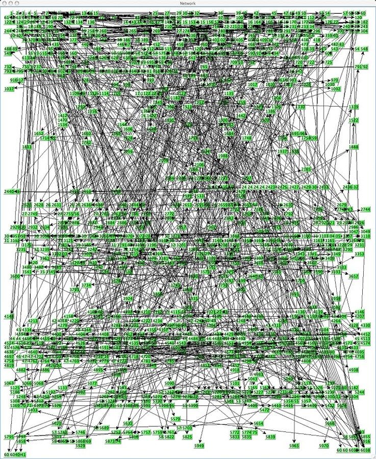
LinkedIn social graph. Blue: cloud computing, Green: big data, dark orange: co-workers, light orange: law school, purple: former employer

Machine Learning Algorithms

Decision trees

K-nearest Neighbour

\hat f(\vec x_q) = \frac{\sum_{i=1}^kw_if(x_i)}{\sum_{i=1}^kw_i}
f^(xq)=i=1kwif(xi)i=1kwi\hat f(\vec x_q) = \frac{\sum_{i=1}^kw_if(x_i)}{\sum_{i=1}^kw_i}
w = \frac{1}{d(x_q, x_i)^2}
w=1d(xq,xi)2w = \frac{1}{d(x_q, x_i)^2}

Linear Regression

p(C_k|\vec x) = \frac{p(\vec x|C_k)p(C_k)}{p(\vec x)}
p(Ckx)=p(xCk)p(Ck)p(x)p(C_k|\vec x) = \frac{p(\vec x|C_k)p(C_k)}{p(\vec x)}

Naive Bayes and Bayesian Networks

\vec x = (x_1, \ldots, x_n)
x=(x1,,xn)\vec x = (x_1, \ldots, x_n)
p(C_k, x_1, \ldots, x_n) = p(C_k)p(x_1, \ldots, x_n |C_k)
p(Ck,x1,,xn)=p(Ck)p(x1,,xnCk)p(C_k, x_1, \ldots, x_n) = p(C_k)p(x_1, \ldots, x_n |C_k)
= p(C_k)p(x_1|C_k)p(x_2, \ldots, x_n |C_k, x_1)
=p(Ck)p(x1Ck)p(x2,,xnCk,x1)= p(C_k)p(x_1|C_k)p(x_2, \ldots, x_n |C_k, x_1)
= p(C_k)p(x_1|C_k)p(x_2|C_k, x_1)p(x_3, \ldots, x_n|C_k, x_1, x_2)
=p(Ck)p(x1Ck)p(x2Ck,x1)p(x3,,xnCk,x1,x2)= p(C_k)p(x_1|C_k)p(x_2|C_k, x_1)p(x_3, \ldots, x_n|C_k, x_1, x_2)
= p(C_k)p(x_1|C_k)p(x_2|C_k, x_1)\ldots p(x_n|C_k, x_1, x_2, x_3, \ldots, x_{n-1})
=p(Ck)p(x1Ck)p(x2Ck,x1)p(xnCk,x1,x2,x3,,xn1)= p(C_k)p(x_1|C_k)p(x_2|C_k, x_1)\ldots p(x_n|C_k, x_1, x_2, x_3, \ldots, x_{n-1})
p(x_i|C_k, x_j) = p(x_i|C_k)
p(xiCk,xj)=p(xiCk)p(x_i|C_k, x_j) = p(x_i|C_k)
p(x_i|C_k, x_j, x_k) = p(x_i|C_k)
p(xiCk,xj,xk)=p(xiCk)p(x_i|C_k, x_j, x_k) = p(x_i|C_k)
p(x_i|C_k, x_j, x_k, x_l) = p(x_i|C_k)
p(xiCk,xj,xk,xl)=p(xiCk)p(x_i|C_k, x_j, x_k, x_l) = p(x_i|C_k)
p(C_k | x_1, \ldots, x_n) \propto p(C_k, x_1, \ldots, x_n)
p(Ckx1,,xn)p(Ck,x1,,xn)p(C_k | x_1, \ldots, x_n) \propto p(C_k, x_1, \ldots, x_n)
\propto p(C_k)p(x_1|C_k)p(x_2|C_k)p(x_3|C_k)\ldots
p(Ck)p(x1Ck)p(x2Ck)p(x3Ck)\propto p(C_k)p(x_1|C_k)p(x_2|C_k)p(x_3|C_k)\ldots
\propto p(C_k)\prod_{i=1}^n p(x_i|C_k)
p(Ck)i=1np(xiCk)\propto p(C_k)\prod_{i=1}^n p(x_i|C_k)

"Naive" conditional independance assumption

p(C_k|x_1, \ldots, x_n)= \frac{1}{Z} p(C_k)\prod_{i=1}^n p(x_i|C_k)
p(Ckx1,,xn)=1Zp(Ck)i=1np(xiCk)p(C_k|x_1, \ldots, x_n)= \frac{1}{Z} p(C_k)\prod_{i=1}^n p(x_i|C_k)
Z = \frac {1}{p(\vec x)}
Z=1p(x)Z = \frac {1}{p(\vec x)}
\hat y = C_k
y^=Ck\hat y = C_k
\hat y = argmax_{k (\in 1, \ldots, K)}p(C_k)\prod_{i=1}^np(x_i|C_k)
y^=argmaxk(1,,K)p(Ck)i=1np(xiCk)\hat y = argmax_{k (\in 1, \ldots, K)}p(C_k)\prod_{i=1}^np(x_i|C_k)

perceptrons and neural Networks

Support Vector Machines (SVM)

< \vec{x}, y >
<x,y>< \vec{x}, y >
\vec{x} \rightarrow f(\vec{x})
xf(x)\vec{x} \rightarrow f(\vec{x})
h \in H : H = \{h_1, h_2, \ldots, h_n\}
hH:H={h1,h2,,hn}h \in H : H = \{h_1, h_2, \ldots, h_n\}
\vec{w} = \{w_1, w_2, \ldots, w_n\}
w={w1,w2,,wn}\vec{w} = \{w_1, w_2, \ldots, w_n\}
f(\vec x) \approx \tilde{f}(\vec x) = \sum_i w_i h_i(\vec x)
f(x)f~(x)=iwihi(x)f(\vec x) \approx \tilde{f}(\vec x) = \sum_i w_i h_i(\vec x)

Supervised Learning: 

Goal

An Example

\vec{w}^* = argmin_{\vec w} \sum_j^{N} (f(\vec x_j) - \sum_i w_ih_i(\vec x_j))^2
w=argminwjN(f(xj)iwihi(xj))2\vec{w}^* = argmin_{\vec w} \sum_j^{N} (f(\vec x_j) - \sum_i w_ih_i(\vec x_j))^2
h \in H : H = \{h_1, h_2, \ldots, h_n\}
hH:H={h1,h2,,hn}h \in H : H = \{h_1, h_2, \ldots, h_n\}
\vec{w} = \{w_1, w_2, \ldots, w_n\}
w={w1,w2,,wn}\vec{w} = \{w_1, w_2, \ldots, w_n\}
f(\vec x) \approx \tilde{f}(\vec x) = \sum_i w_i h_i(\vec x)
f(x)f~(x)=iwihi(x)f(\vec x) \approx \tilde{f}(\vec x) = \sum_i w_i h_i(\vec x)

Linear Regression

< x_i, d_i >
<xi,di>< x_i, d_i >
d_i = f(\vec x) + \epsilon_i
di=f(x)+ϵid_i = f(\vec x) + \epsilon_i
\epsilon_i \sim N(0, \sigma_{\epsilon})
ϵiN(0,σϵ)\epsilon_i \sim N(0, \sigma_{\epsilon})
h_{ML} = argmax_{h \in H} P(D|h) = \prod_i^m p(d_i | h)
hML=argmaxhHP(Dh)=imp(dih) h_{ML} = argmax_{h \in H} P(D|h) = \prod_i^m p(d_i | h)
p(d_i | h) = \frac{1}{\sqrt{2\pi\sigma^2}}e^{-\frac{1}{2}(\frac{d_i - h(x_i)}{\sigma})^2}
p(dih)=12πσ2e12(dih(xi)σ)2p(d_i | h) = \frac{1}{\sqrt{2\pi\sigma^2}}e^{-\frac{1}{2}(\frac{d_i - h(x_i)}{\sigma})^2}
h_{ML} = argmax_{h \in H} \sum_i^m ln(\frac{1}{\sqrt{2\pi\sigma^2}}) - (\frac{1}{2}\frac{d_i - h(x_i)}{\sigma})^2
hML=argmaxhHimln(12πσ2)(12dih(xi)σ)2 h_{ML} = argmax_{h \in H} \sum_i^m ln(\frac{1}{\sqrt{2\pi\sigma^2}}) - (\frac{1}{2}\frac{d_i - h(x_i)}{\sigma})^2
h_{ML} = argmax_{h \in H} \sum_i^m - (d_i - h(x_i))^2
hML=argmaxhHim(dih(xi))2 h_{ML} = argmax_{h \in H} \sum_i^m - (d_i - h(x_i))^2
h_{ML} = argmin_{h \in H} \sum_i^m (d_i - h(x_i))^2
hML=argminhHim(dih(xi))2 h_{ML} = argmin_{h \in H} \sum_i^m (d_i - h(x_i))^2
Bias = E[\hat f(\vec x)] - f(\vec x)
Bias=E[f^(x)]f(x)Bias = E[\hat f(\vec x)] - f(\vec x)
  • Measures how well you expect to represent the "true" solution
  • Decreases with model complexity

Learning Bias

Variance = E[(\hat f(\vec x) - E [\hat f(\vec x)]]^2
Variance=E[(f^(x)E[f^(x)]]2Variance = E[(\hat f(\vec x) - E [\hat f(\vec x)]]^2
  • Measures how sensitive given learner is to a specific dataset 
  • Decreases with simpler model

Learning Variance

Simple models may not fit the data


Complex models may not be applicable to new, as of yet unseen data

choice of hypothesis class introduces learning bias


more complex class, less bias, but more variance

Bias-Variance Tradeoff

Error can be decomposed:

Err(\vec x) = E[(f(\vec x) - \hat f(\vec x))^2]
Err(x)=E[(f(x)f^(x))2]Err(\vec x) = E[(f(\vec x) - \hat f(\vec x))^2]
= (E[\hat f(\vec x)] - f(\vec x))^2 + E[(\hat f(\vec x) - E [\hat f(\vec x)]]^2 + \sigma^2
=(E[f^(x)]f(x))2+E[(f^(x)E[f^(x)]]2+σ2= (E[\hat f(\vec x)] - f(\vec x))^2 + E[(\hat f(\vec x) - E [\hat f(\vec x)]]^2 + \sigma^2

Choice of hypothesis class introduces learning bias

Bias-Variance Tradeoff

= Bias^2 + Variance + \sigma^2
=Bias2+Variance+σ2= Bias^2 + Variance + \sigma^2

Overfitting

Training Set Error:

error_{train}(\vec w) = \frac{1}{N_t}\sum_{j=1}^{N_t}(f(\vec x_j) - \sum_i w_ih_i(\vec x_j))^2
errortrain(w)=1Ntj=1Nt(f(xj)iwihi(xj))2error_{train}(\vec w) = \frac{1}{N_t}\sum_{j=1}^{N_t}(f(\vec x_j) - \sum_i w_ih_i(\vec x_j))^2

Overfitting

error_{true}(\vec w) = \int_x(f(\vec x) - \sum_i w_ih_i(\vec x))^2p(x)dx
errortrue(w)=x(f(x)iwihi(x))2p(x)dxerror_{true}(\vec w) = \int_x(f(\vec x) - \sum_i w_ih_i(\vec x))^2p(x)dx
error_{true}(\vec w) \approx \frac{1}{M}\sum_{j=1}^{M}(f(\vec x_j) - \sum_i w_ih_i(\vec x_j))^2
errortrue(w)1Mj=1M(f(xj)iwihi(xj))2error_{true}(\vec w) \approx \frac{1}{M}\sum_{j=1}^{M}(f(\vec x_j) - \sum_i w_ih_i(\vec x_j))^2

Prediction Error:

error_{true}(\vec w) \approx \frac{1}{M}\sum_{j=1}^{M}(f(\vec x_j) - \sum_i w_ih_i(\vec x_j))^2
errortrue(w)1Mj=1M(f(xj)iwihi(xj))2error_{true}(\vec w) \approx \frac{1}{M}\sum_{j=1}^{M}(f(\vec x_j) - \sum_i w_ih_i(\vec x_j))^2
error_{train}(\vec w) = \frac{1}{N_t}\sum_{j=1}^{N_t}(f(\vec x_j) - \sum_i w_ih_i(\vec x_j))^2
errortrain(w)=1Ntj=1Nt(f(xj)iwihi(xj))2error_{train}(\vec w) = \frac{1}{N_t}\sum_{j=1}^{N_t}(f(\vec x_j) - \sum_i w_ih_i(\vec x_j))^2

Why doesn't training error approximate prediction error?

training error good estimate for single w, but w was optimised with respect to training data, and found that w was good for this set of samples

Generalisation

Test Set Error

error_{test}(\vec w) = \frac{1}{N_{test}}\sum_{j=1}^{N_{test}}(f(\vec x_j) - \sum_i w_ih_i(\vec x_j))^2
errortest(w)=1Ntestj=1Ntest(f(xj)iwihi(xj))2error_{test}(\vec w) = \frac{1}{N_{test}}\sum_{j=1}^{N_{test}}(f(\vec x_j) - \sum_i w_ih_i(\vec x_j))^2

Given dataset D, randomly split into two parts:

  • Training data
  • Test data

Use Training Data to optimise w

For the final output w', evaluate error once using:  

Generalisation

A learning algorithm overfits the training data if it outputs a solution w' when there exists another solution w'' such that:

[error_{train}(w') < error_{train}(w'')] \wedge [error_{test}(w'') < error_{test}(w')]
[errortrain(w)<errortrain(w)][errortest(w)<errortest(w)][error_{train}(w') < error_{train}(w'')] \wedge [error_{test}(w'') < error_{test}(w')]

Overfitting typically leads to very large parameter choices


Regularised regression aims to impose a complexity restriction by penalising large weights

Generalisation

better on training data

worse on testing data

\hat{w}_{ridge} = argmin_w \sum_{j=1}^N(f(\vec x_j) - (w_0 + \sum_i^kw_ih_i(\vec x_j)))^2 + \lambda\sum_i^kw_i^2
w^ridge=argminwj=1N(f(xj)(w0+ikwihi(xj)))2+λikwi2\hat{w}_{ridge} = argmin_w \sum_{j=1}^N(f(\vec x_j) - (w_0 + \sum_i^kw_ih_i(\vec x_j)))^2 + \lambda\sum_i^kw_i^2
\hat{w}_{ridge} = argmin_w \sum_{j=1}^N(f(\vec x_j) - (w_0 + \sum_i^kw_ih_i(\vec x_j)))^2 + \lambda\sum_i^k|w_i|
w^ridge=argminwj=1N(f(xj)(w0+ikwihi(xj)))2+λikwi\hat{w}_{ridge} = argmin_w \sum_{j=1}^N(f(\vec x_j) - (w_0 + \sum_i^kw_ih_i(\vec x_j)))^2 + \lambda\sum_i^k|w_i|
\lambda \ge 0
λ0\lambda \ge 0

Ridge Regression

Lasso Regression

Regularisation

Larger 

more penalty, smoother function, more bias

Smaller 

more flexible, more variance

Regularisation

\lambda
λ\lambda
\lambda
λ\lambda

Randomly divide data into k equal parts

D_1, \ldots, D_k
D1,,DkD_1, \ldots, D_k
error_{D_i} = \frac{k}{N} \sum_{\vec x_j \in D_i} (f(\vec x_j) - h_{\frac{D}{D_i}}(\vec x_j))^2
errorDi=kNxjDi(f(xj)hDDi(xj))2error_{D_i} = \frac{k}{N} \sum_{\vec x_j \in D_i} (f(\vec x_j) - h_{\frac{D}{D_i}}(\vec x_j))^2

Learn classifier

h_{\frac{D}{D_i}}
hDDih_{\frac{D}{D_i}}

Estimate error of 

h_{\frac{D}{D_i}}
hDDih_{\frac{D}{D_i}}

on validation set

D_i
DiD_i

k-Fold Cross Validation

using data not in

D_i
DiD_i
error_{k-fold} = \frac{1}{k}\sum_{i=1}^kerror_{D_i}
errorkfold=1ki=1kerrorDierror_{k-fold} = \frac{1}{k}\sum_{i=1}^kerror_{D_i}

ML Pipeline

END PROGRAM.

Made with Slides.com