Model Predictive Control for
Legged Robots
Niraj Rathod
Computer Science and Systems Engineering, XXXIII Cycle
PhD defense

Prof. Alberto Bemporad
Advisors
IMT School for Advanced Studies Lucca, Italy
Dr. Michele Focchi
DLS Lab, Istituto Italiano di Tecnologia, Genova, and
University of Trento, Italy
Assoc. Prof. Mario Zanon
IMT School for Advanced Studies Lucca, Italy
Why Legged Robots?
Agile
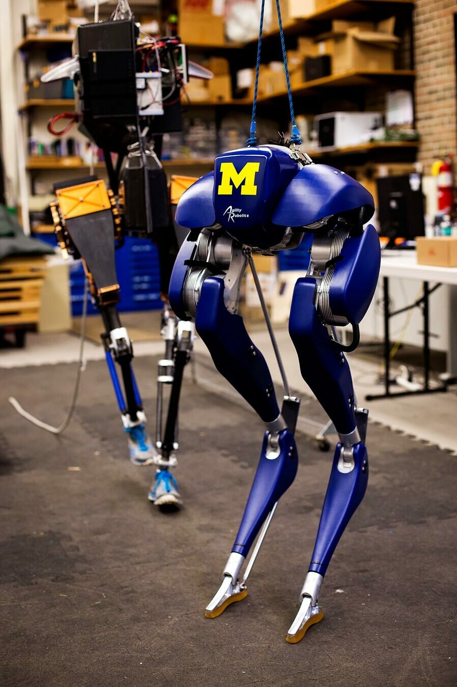
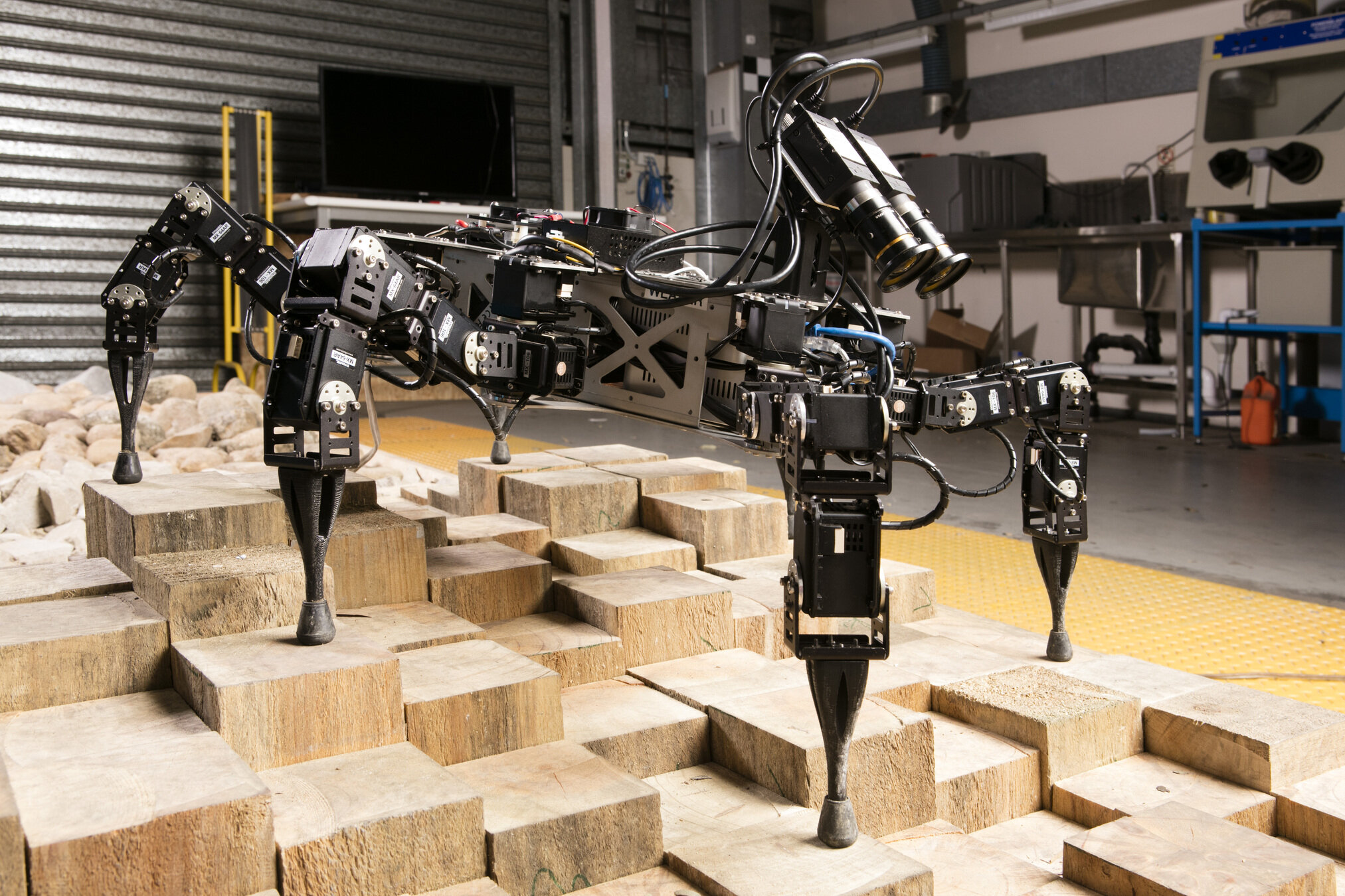
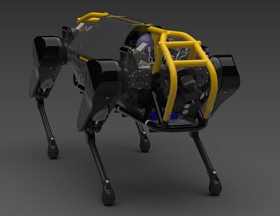
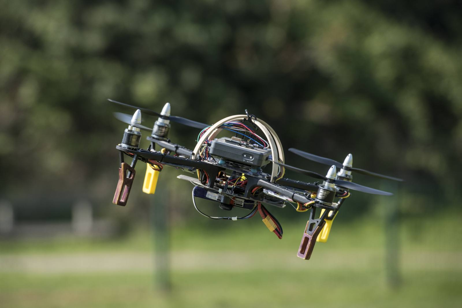
Strong
source:https://www.youtube.com/embed/tF4DML7FIWk?enablejsapi=1
source:https://youtu.be/pLsNs1ZS_TI
Cassie: https://news.engin.umich.edu/2017/09/latest-two-legged-walking-robot-arrives-at-michigan/
Hexaped: https://www.csiro.au/en/research/
HyQReal: https://dls.iit.it/web/dynamic-legged-systems/robots
sources:
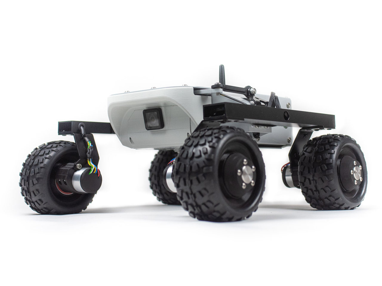
Wheeled robot: https://www.leorover.tech/post/top-3-ways-to-set-a-robot-into-motion
Quadrotor: http://uosdesign.org/designshow2015/ni-myrio-autonomous-quadrotor/
sources:
Objective of this thesis
Robot
Task
Environment
Generate motion plan
Optimal control techniques



Model predictive control with environment adaptation for legged locomotion, IEEE Access, vol. 9, pp. 145710-145727, 2021
Optimization-Based Reference Generator for Nonlinear Model Predictive Control of Legged Robots. Robotics 2023, 12(1), 6, 2023
?
Outline
Outline
Model Validation


Outline
Model Validation
Trajectory Optimization for Legged Locomotion


Outline
Model Validation
Trajectory Optimization for Legged Locomotion
Nonlinear Model Predictive Control


Outline
Model Validation
Nonlinear Model Predictive Control
Two-Stage Optimization


Trajectory Optimization for Legged Locomotion
Model validation
Model selection for optimal planning
High fidelity model
Rigid Body Dynamics
- Accurate
- Good for simulators and offline Trajectory Optimization

- Might be unsuitable for real-time optimal planning
Model selection for optimal planning
High fidelity model
Rigid Body Dynamics
- Accurate
- Good for simulators and offline Trajectory Optimization

- Might be unsuitable for real-time optimal planning
Approximate Model
Single Rigid Body Dynamics
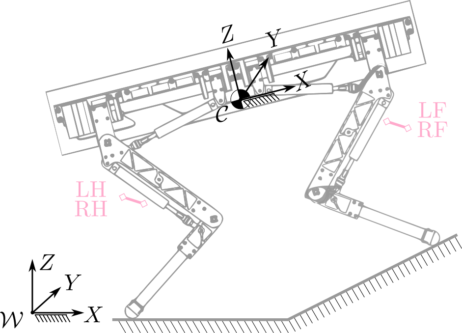
- Includes linear and angular dynamics
- Suitable for real-time optimal planning
- Less accurate
Robot model
Single Rigid Body Dynamics (SRBD)
Discrete-time state space model
Linear time-varying model
Continuous-time state space model
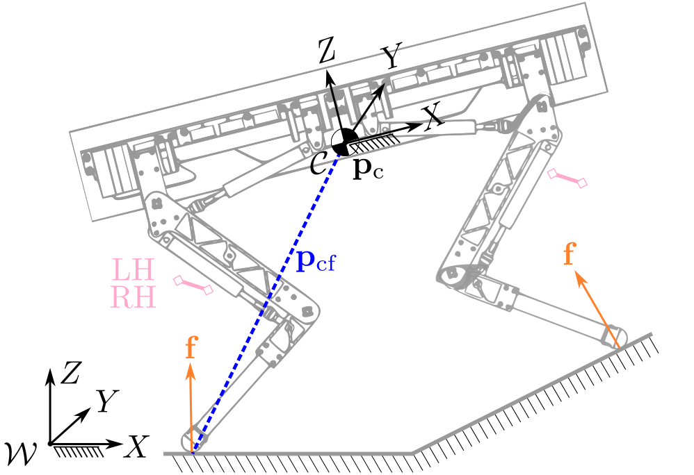
- The SRBD model is nonlinear with the unstable dynamics
- Therefore, it requires a stabilizing controller to simulate a nominal working condition
Closed-loop system validation
Why closed-loop system validation?
Closed-loop system validation
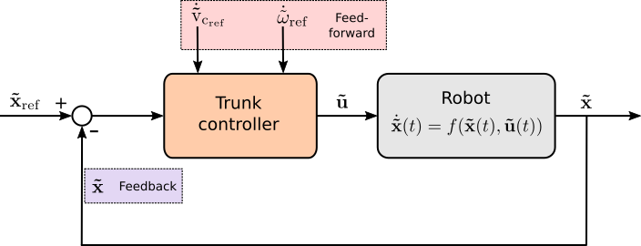
Approximate model
For model validation:
validated by
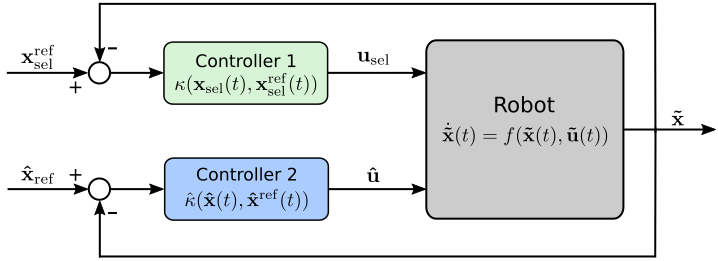
Validation results
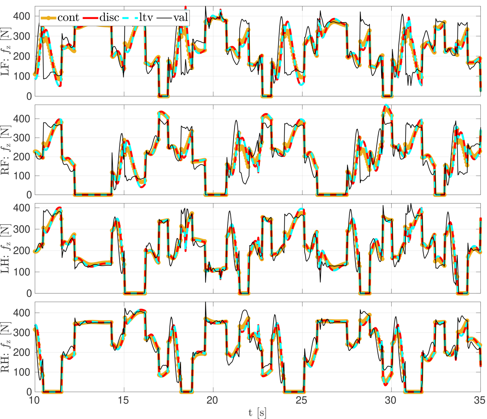
Validation data: HyQ crawling with the body pitch and yaw
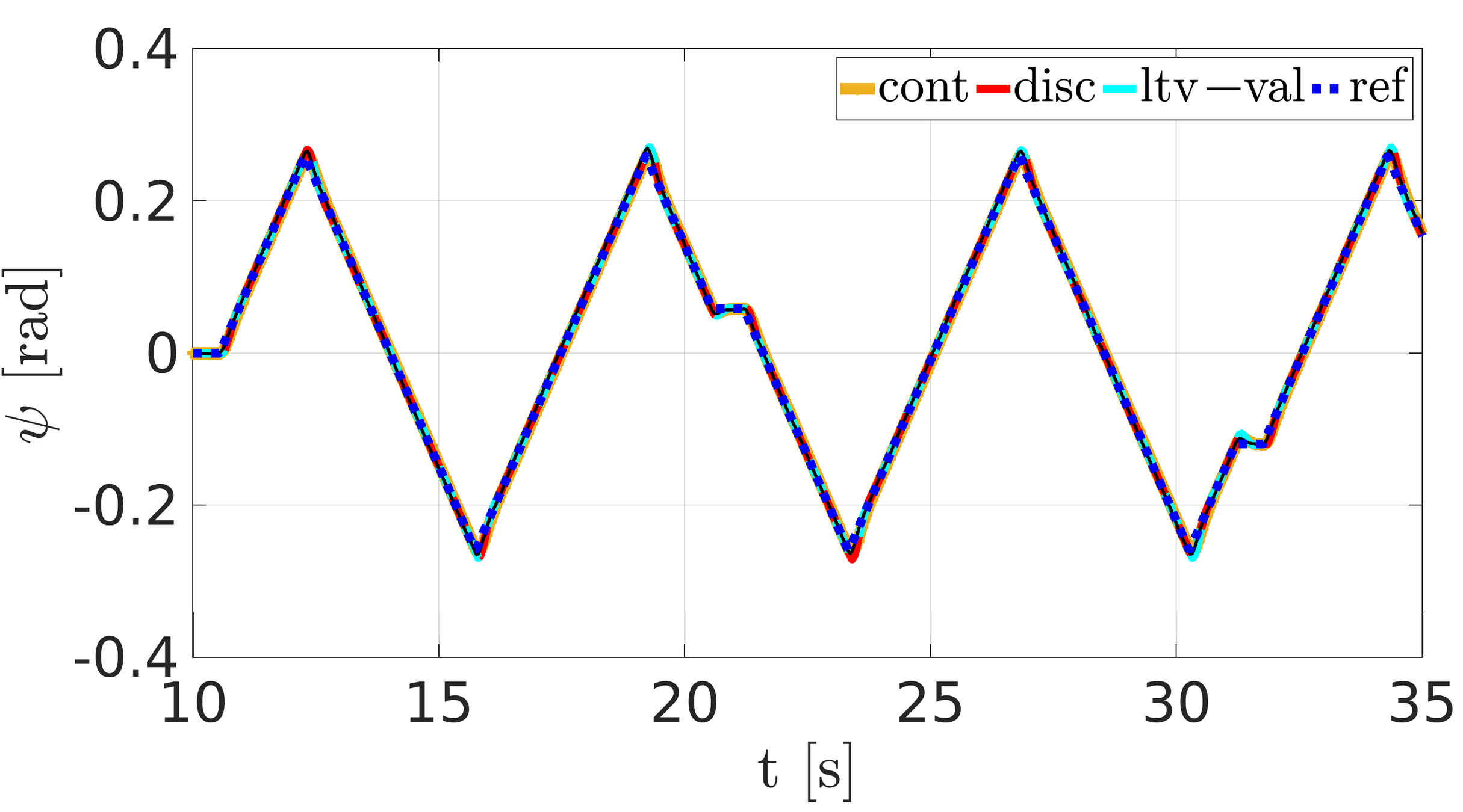
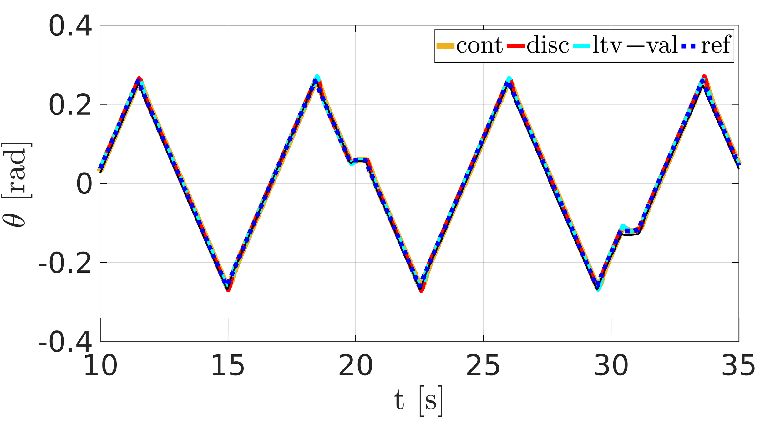
Pitch
yaw
Ground reaction forces for pitch validation
Trajectory Optimization for Legged Locomotion
Trajectory Optimization: LTVOpt
LTV form of the SRBD model
Friction cone and unilateral constraints
Reference \(\mathbf{x}^\mathrm{ref}\) and \(\mathbf{u}^\mathrm{ref}\) generation from heuristic
State \(\mathbf{x}\) and Input \(\mathbf{u}\) tracking term
Uses references (often dynamically infeasible) as linearization trajectory to obtain LTV model
The solution of the LTVOpt may be dynamically infeasible
Initial condition
So the proposed solution is ...
Trajectory Optimization: SQPOpt
- Gives dynamically feasible solution if converged
- LTV form of the SRBD model
- Quadratic cost: State \(\mathbf{x}\) and Input \(\mathbf{u}\) tracking term
- Usually solves more than one QP in a single run therefore can be computationally demanding
- Friction cone and unilateral constraints
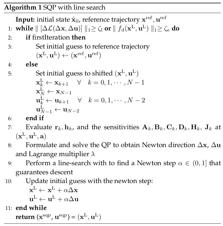
Back Tracking Algorithm
Results: LTVOpt and SQPOpt


CoM position
CoM velocity
- Prediction horizon: 4 s (100 nodes)
- Sampling time 40 ms
- Solver: Gurobi
- Solution time:
- LTVOpt : 200 ms
- SQPOpt : 1-1.2 s
Implementation details:
Results: LTVOpt and SQPOpt

Ground reaction forces: normal components


Orientation
Angular velocity
Nonlinear Model Predictive Control
Why NMPC?
- Many successful MPC implementation [1], [2], [3] examples in legged locomotion
- Some MPC implementation either neglect angular dynamics [4] or linearize it [5] that is not good for large variation from the horizontal orientation
- We would like to facilitate locomotion that involves considerable base orientation
- NMPC unlike linear MPC allows one to include nonlinear dynamics, non-quadratic cost and nonlinear inequalities
[1] J. Koenemann, et al. Whole-body model-predictive control applied to the HRP-2 humanoid. In IEEE/RSJ Int. Conf. Intell. Robot. Syst., pages 3346–3351, 2015.
[2 ] M. Neunert, et al. Whole-Body Nonlinear Model Predictive Control Through Contacts for Quadrupeds. IEEE Robot. Autom. Lett., 3(3):1458–1465,2018.
[3] R. Grandia, et al. Feedback mpc for torque controlled legged robots. In 2019 IEEE/RSJ International Conference on Intelligent Robots and Systems (IROS), pages 4730–4737, 2019.
[4] A. Herdt, et al. Online walking motion generation with automatic footstep placement. Advanced Robotics, 24(5-6):719–737, 2010.
[5] J. Di Carlo, et al. Dynamic locomotion in the MIT cheetah 3 through convex model-predictive control. In 2018 IEEE/RSJ International Conference on Intelligent Robots and Systems (IROS), pages 1–9,2018.
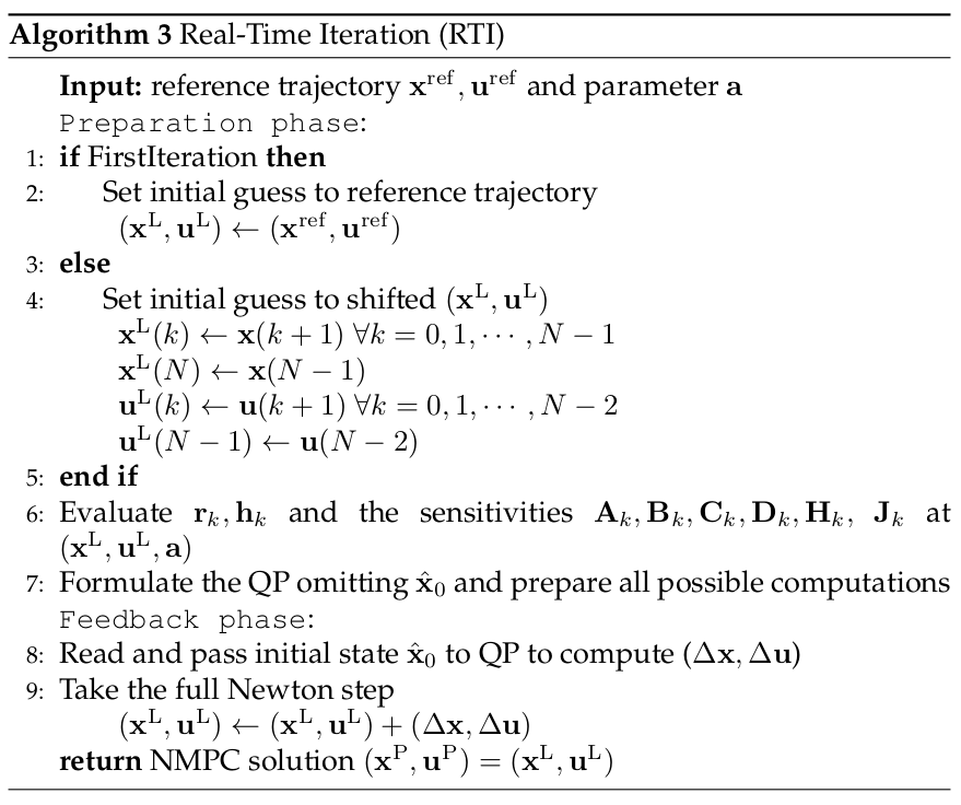
Towards Real-Time Iteration scheme
- Since LTVOpt solves one QP at each call it is faster than SQPOpt
- LTVOpt uses reference as linearization trajectory whereas SQPOpt warm starts after the first iteration
- SQPOpt solves until convergence thus can provide feasible solution
- To solve only one QP online
- To warm start from the previous solution to evaluate the sensitivities in the next call of the algorithm
We use Real-Time Iteration (RTI) scheme for our NMPC.
For online implementation it is desirable:
Locomotion framework

NMPC runs at \( 25\, \mathrm{Hz} \)
WBC runs at \( 250\, \mathrm{Hz} \)
State estimator runs at \( 500\, \mathrm{Hz} \)
Joint Space PD runs at \( 1\, \mathrm{kHz} \)
Grid map runs at \( 30\, \mathrm{Hz} \)
NMPC formulation
State \(\mathbf{x}_k \in \mathbb{R}^{12} \)
vector of the robot's CoM position, CoM velocity, base orientation, and angular velocity
Control input \(\mathbf{u}_k \in \mathbb{R}^{12} \)
vector of ground reaction forces
vector of foot locations and contact status
Model parameters \(\mathbf{a}_k \in \mathbb{R}^{16} \)
Decision variables:
Predicted state \(\mathbf{x}^\mathrm{p}=\{\mathbf{x}_{0}, \ldots, \mathbf{x}_N\}\)
Control inputs \(\mathbf{u}^\mathrm{p}=\{\mathbf{u}_{0}, \ldots, \mathbf{u}_{N-1}\}\)
Nonlinear Programming problem

Cost function
- \(\ell_\mathrm{t}\) is tracking cost on \(\mathbf{x}_k \in \mathbb{R}^{12} \) and control inputs \(\mathbf{u}_k \in \mathbb{R}^{12} \)
- \(\ell_\mathrm{r}\) is the regularization term for the control inputs to keep contact normal as close to the center of the friction cone
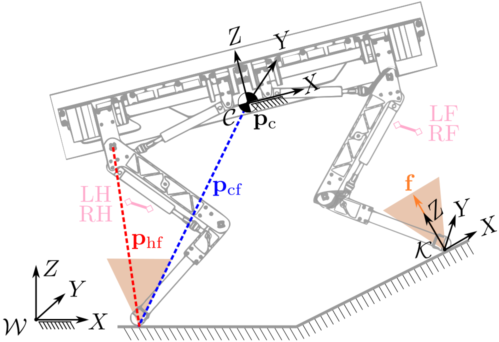
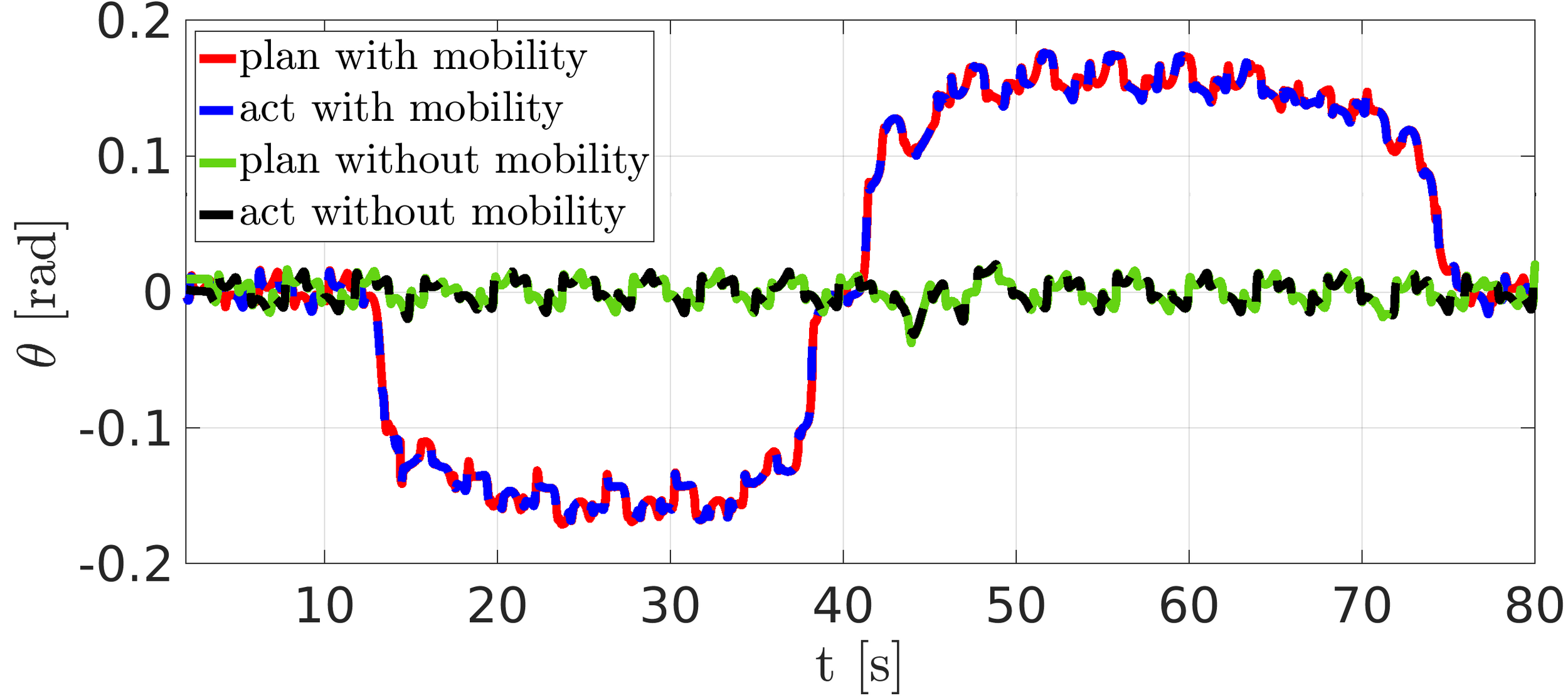
- \(\ell_\mathrm{m}\) is the mobility cost that penalizes hip-to-foot distance from the reference
SRBD Model for NMPC
- Defined in the CoM frame, so constant inertia
- Binary parameters \(\delta_i = \{0, 1\}\) to define whether foot \(i\) is in contact with the ground

Defined in the CoM frame
Included \(\delta_i\)
Mobility
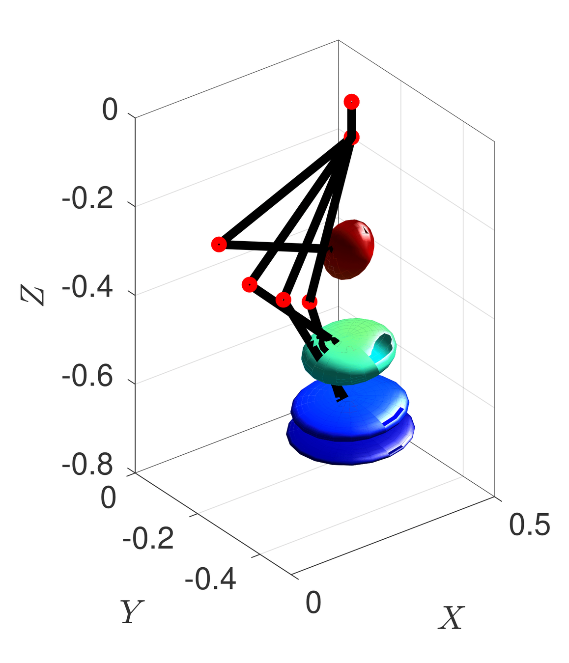
- Parameters \(\beta\) and \(\gamma\) are introduced to find the best trade-off between the volume and eccentricity
- Mobility factor \(l_\mathrm{m}\) can be evaluated inside the workspace of each leg
- This analysis outputs the hip-to-foot distance belonging to the highest mobility that is used as a reference for the mobility cost inside the NMPC
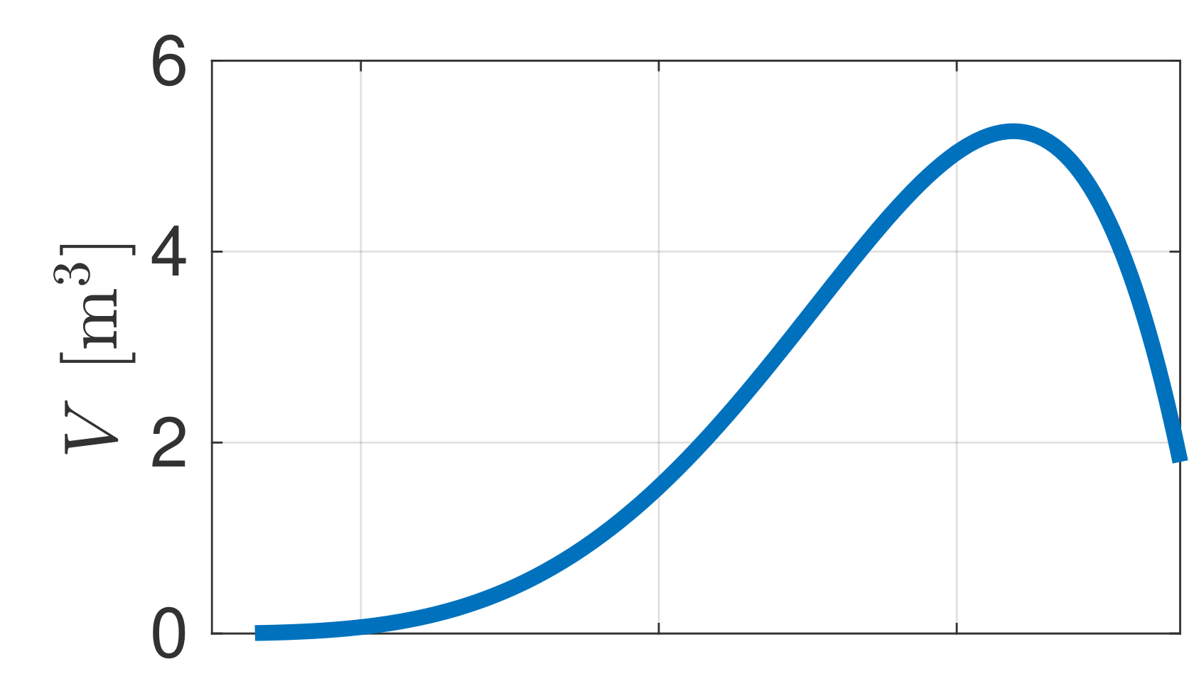

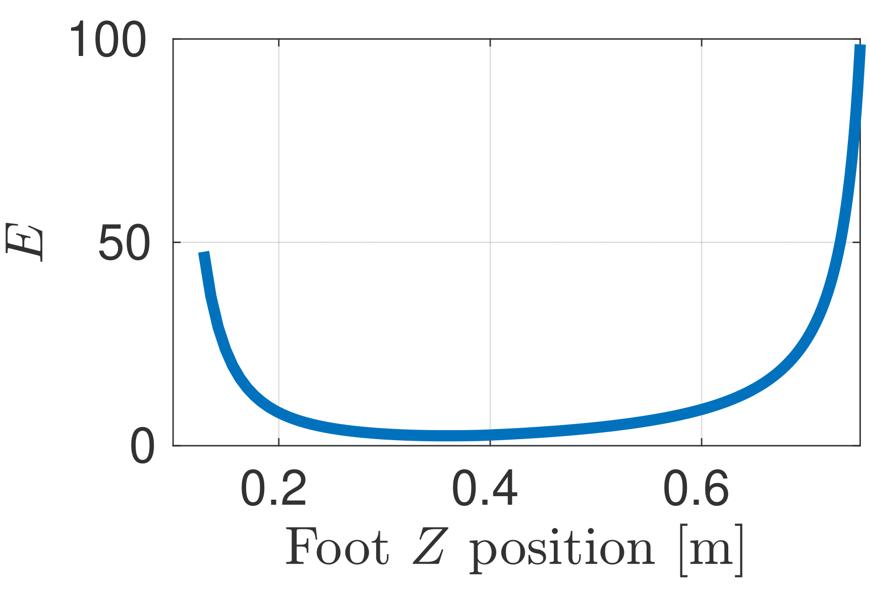
Simulation: NMPC with mobility
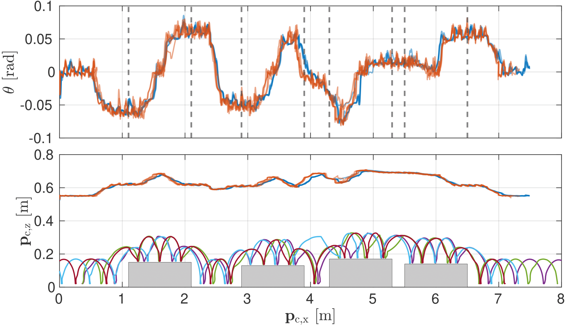
Simulation: NMPC with pallet crossing
Simulation: NMPC with force robustness
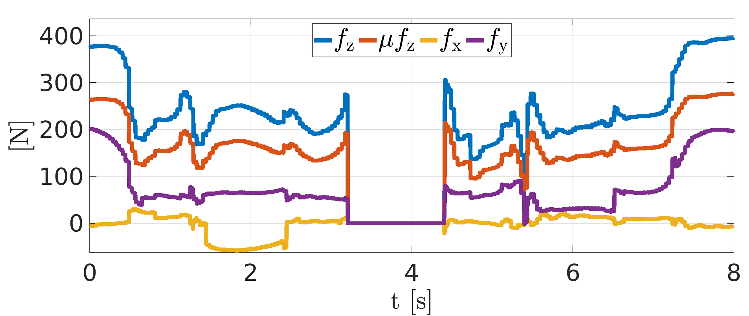
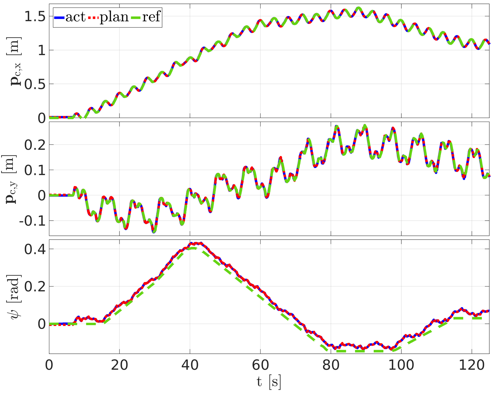
Experiment: NMPC omni-directional walk
Experiments: NMPC with traversing pallets
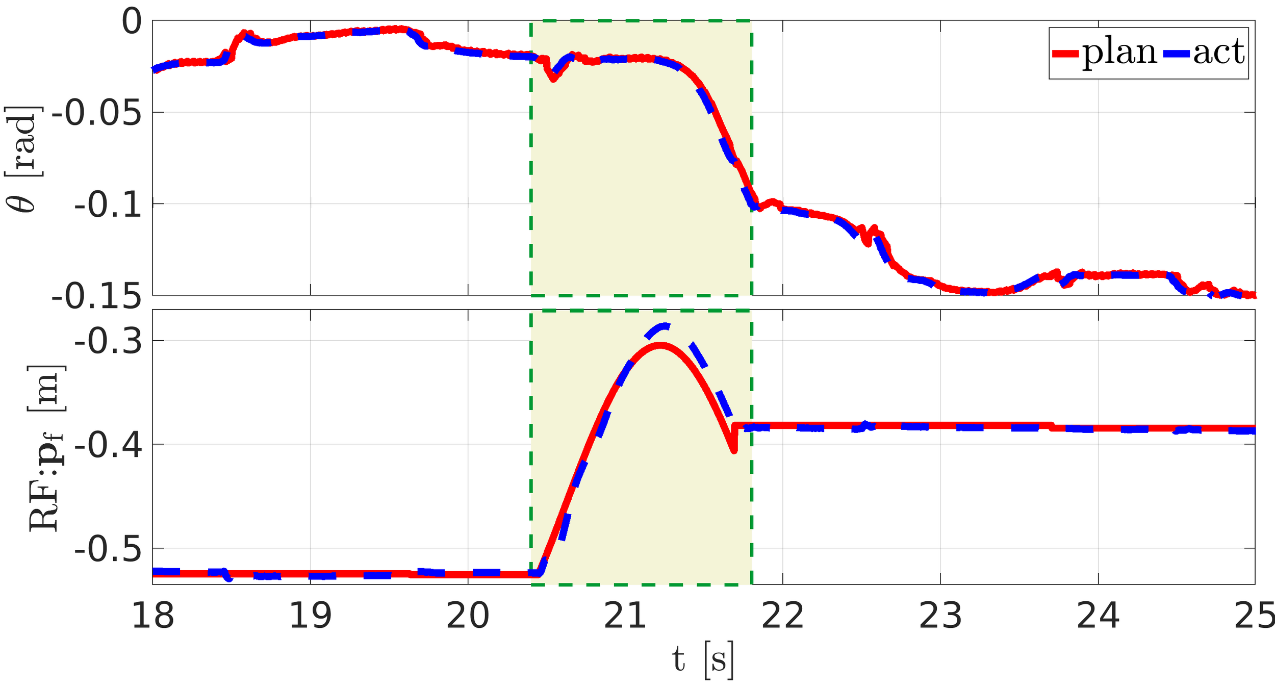
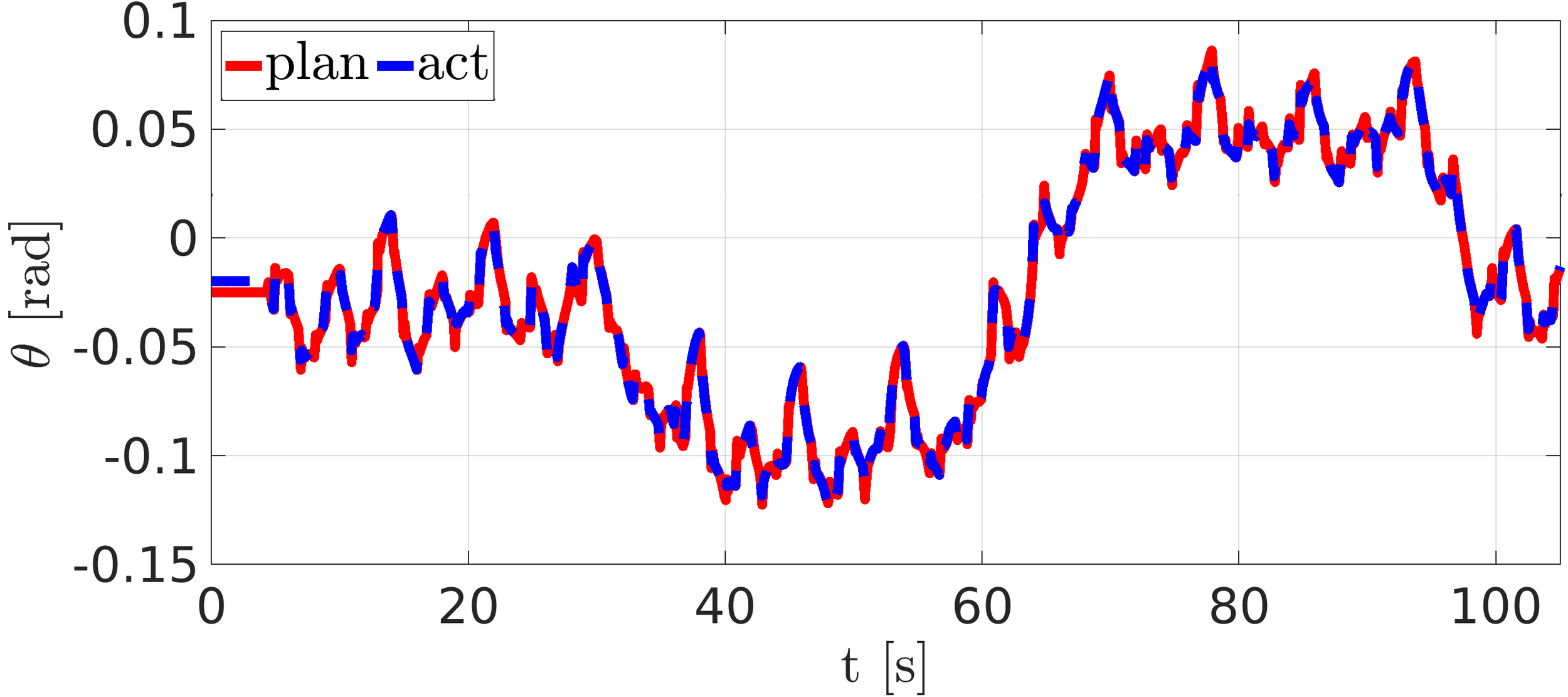
Static pallet
Repositioned pallet
Experiments: Trotting in a straight line
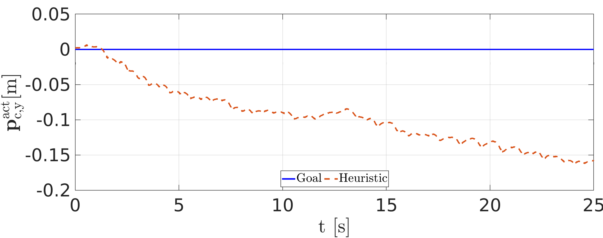
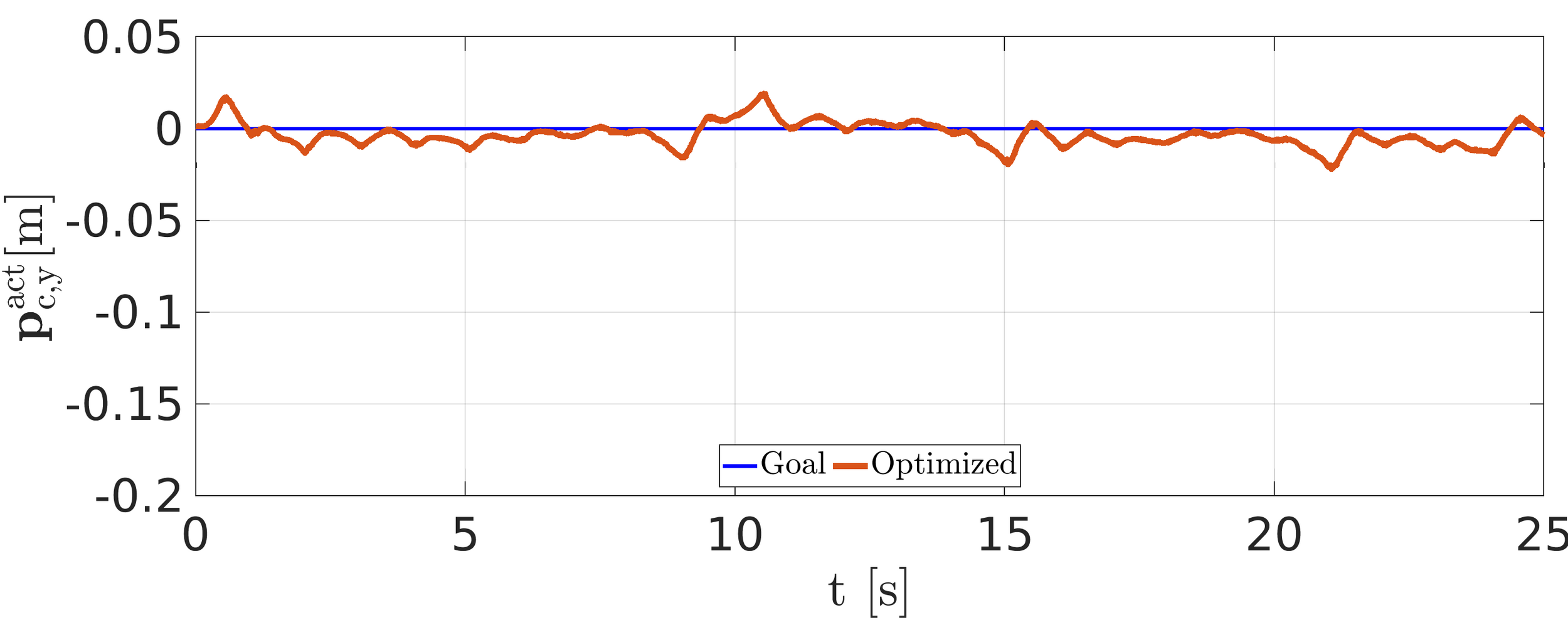
Two-Stage Optimization
Optimization-based reference generator
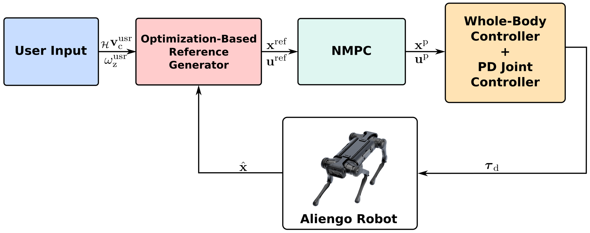
- Provides physically informed reference trajectory to the NMPC
- Computes the foothold heuristically coherent with the CoM position
Why is it needed?
- Takes care of the underactuation of statically unstable gaits like trot
- Allows to cope with the external disturbances
Optimization-based reference generator

NMPC
LIP model optimization
QP mapping
+
Remaining state from heuristics
Simulation: pace gait
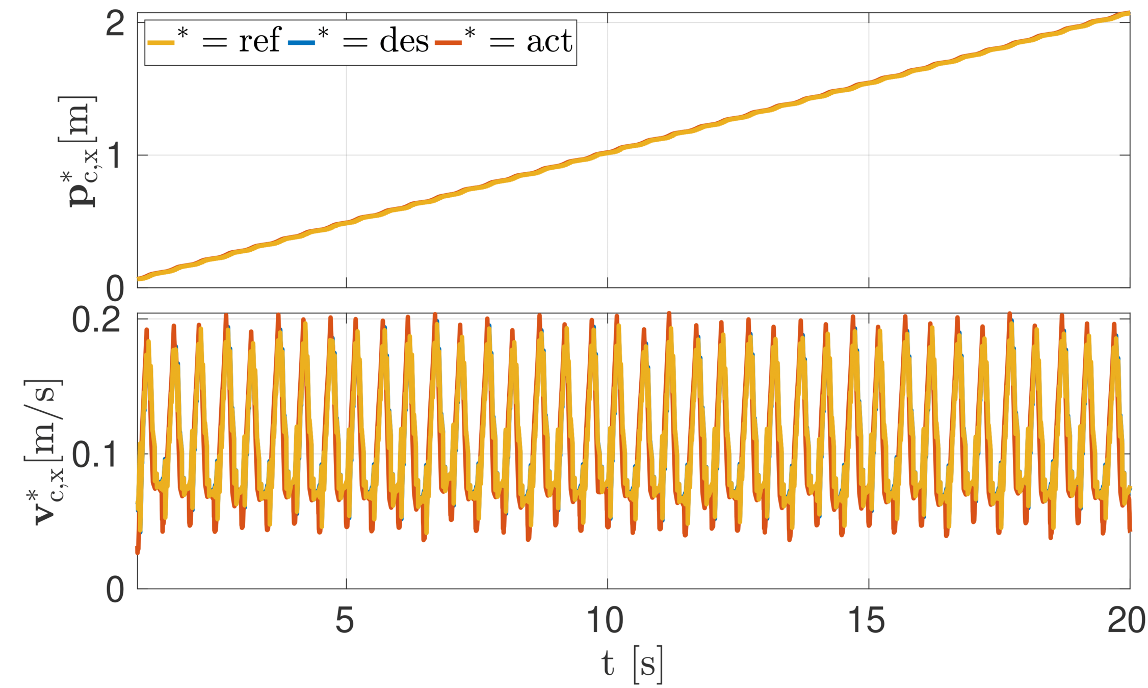
Experiment: trotting in a straight line
Experiment: recovery from external pushes
Summary and future directions
Summary
- Model validation of the SRBD model
- Introduced two Trajectory optimization schemes
- Nonlinear Model Predictive Control with leg mobility
- Two-Stage Optimization: NMPC with optimal reference generator
- LTVOpt
- SQPOpt
Future directions
- Auto-tuning algorithm to tune the NMPC weights
- Extend our NMPC formulation to optimize the step timing and foot locations
- NMPC with nonuniform grid discretization method
- A comparative study of linear MPC, LTV-MPC, and NMPC for legged locomotion
Publications
N. Rathod, A. Bratta, M. Focchi, M. Zanon, O. Villarreal, C. Semini, A. Bemporad, “Model Predictive Control with Environment Adaptation for Legged Locomotion”, IEEE Access, vol. 9, pp. 145710-145727, 2021.
A. Bratta, M. Focchi, N. Rathod, and C. Semini, “Optimization-Based Reference Generator for Nonlinear Model Predictive Control of Legged Robots”, Robotics 2023, 12(1), 6, 2023.
Journal papers
A. Bratta, N. Rathod, M. Zanon, O. Villarreal, A. Bemporad, C. Semini, M. Focchi, “Towards a Nonlinear Model Predictive Control for Quadrupedal Locomotion on Rough Terrain”, Italian Institute of Robotics and Intelligent Machines (I-RIM) Conference, 3rd edition, Rome, Italy, 2021.
Conference proceedings and workshops
N. Rathod, M. Focchi, M. Zanon, A. Bemporad, “Optimal control based replanning for Quadruped robots”, Numerical Optimization for Online Multi Contact Planning and Control, Robotics: Science and Systems, Freiburg, Germany, 2019.
N. Rathod, A. Bratta, M. Focchi, M. Zanon, O. Villarreal, C. Semini, A. Bemporad, “Real-time MPC with Mobility enhanced Feature for Legged Locomotion”, Towards Real-World Deployment of Legged Robots, ICRA, Xi’an China, 2021.
[2021 IEEE Access Best Video Award (Part 2)]
[Finalist for the Best Student Paper Award]
Collaborators
Claudio Semini
Head of the Dynamic Legged Systems (DLS) research line
Senior Researcher Tenured - Principal Investigator
Istituto Italiano di Tecnologia, Genova
Angelo Bratta
Postdoctoral Researcher at Dynamic Legged Systems lab, Istituto Italiano di Tecnologia, Genova
Octavio Villarreal
Senior Robotics Research Controls Engineer Dyson
City of Bristol, England, United Kingdom