Recap: List of Topics
Descriptive Statistics
Probability Theory
Inferential Statistics
Different types of data
Different types of plots
Measures of centrality and spread
Counting, Sample spaces, events
Discrete and continuous RVs
Bernoulli, Uniform, Normal dist.
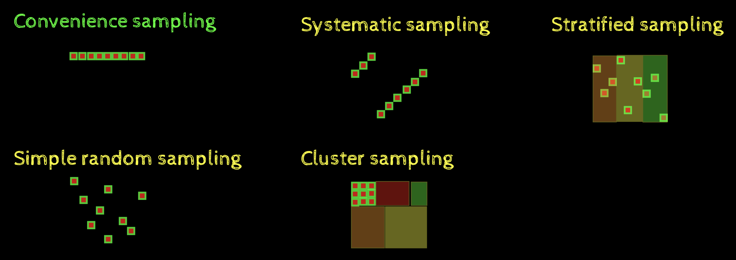
Sampling strategies
Point and Interval Estimators
Hypothesis testing (z-test, t-test)
Chi-square test
Distribution of Sample Statistics
What do we know so far?
How to collect good samples?
What are the distributions of sample statistics?
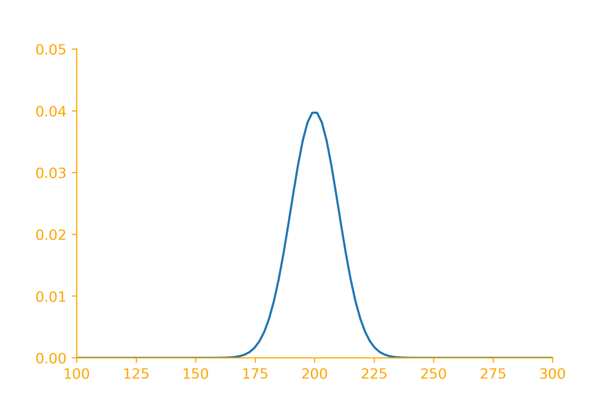
e.g. sample means follow a normal distribution when variance is known

What do we know so far?
if we take different samples from the same population we may get different means

in practice, we have the liberty of taking only one sample
Goal: Make assertions about the population parameters based on sample statistics
Case studies
A company selling chips claims that each packet has 200 grams of chips (as mentioned on the label). You are sceptic of their claims and believe that on average each packet does not contain 200 grams of chips. How will you prove your claim?
Known (status quo):
\mu = 200
Your claim:
\mu \neq 200
Null hypothesis
Alternative hypothesis
How do you test your hypothesis?
Take a sample of n packets
Compute mean weight
Now what?
A company selling chips claims that each packet has 200 grams of chips (as mentioned on the label). You are sceptic of their claims and believe that on average each packet does not contain 200 grams of chips. How will you prove your claim?
\mu = 200
\mu \neq 200
Null hypothesis
Alternative hypothesis
Suppose the mean of the sample is 190 grams, can you conclude that the company is cheating?
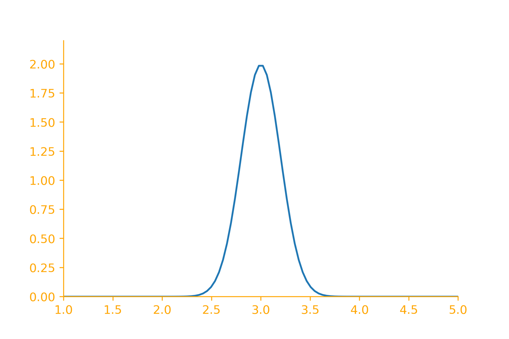
Not always! because we know that the sample means follow a distribution
It is possible to get a sample whose mean is 190 even if the population mean is 200?
How likely is it to get such a mean if the true population mean is 200?
(figuring this out is the goal of this lecture)
If it is very unlikely then reject the null hypothesis
known (status quo)
a bold claim
A company manufacturing ball bearing claims that the average radius of the ball bearings is 3 mm? Your company purchases these ball bearings and has asked you to verify this claim. How will you go about verifying this?
How do you test your hypothesis?
Take a sample of n ball bearings
Compute mean radius
Now what?
\mu = 3
\mu \neq 3
Null hypothesis
Alternative hypothesis
status quo*
a bold claim
* there is no surprise in this as the company already claims this
Suppose the mean of the sample is 3.1 mm, can you conclude that the ball bearings are not suitable?
Not always! because we know that the sample means follow a distribution
It is possible to get a sample whose mean is 3.1 even if the population mean is 3?
How likely is it to get such a mean if the true population mean is 3?
(figuring this out is the goal of this lecture)
If it is very unlikely then reject the null hypothesis
A company manufacturing ball bearing claims that the average radius of the ball bearings is 3 mm? Your company purchases these ball bearings and has asked you to verify this claim. How will you go about verifying this?
\mu = 3
\mu \neq 3
Null hypothesis
Alternative hypothesis
status quo*
a bold claim
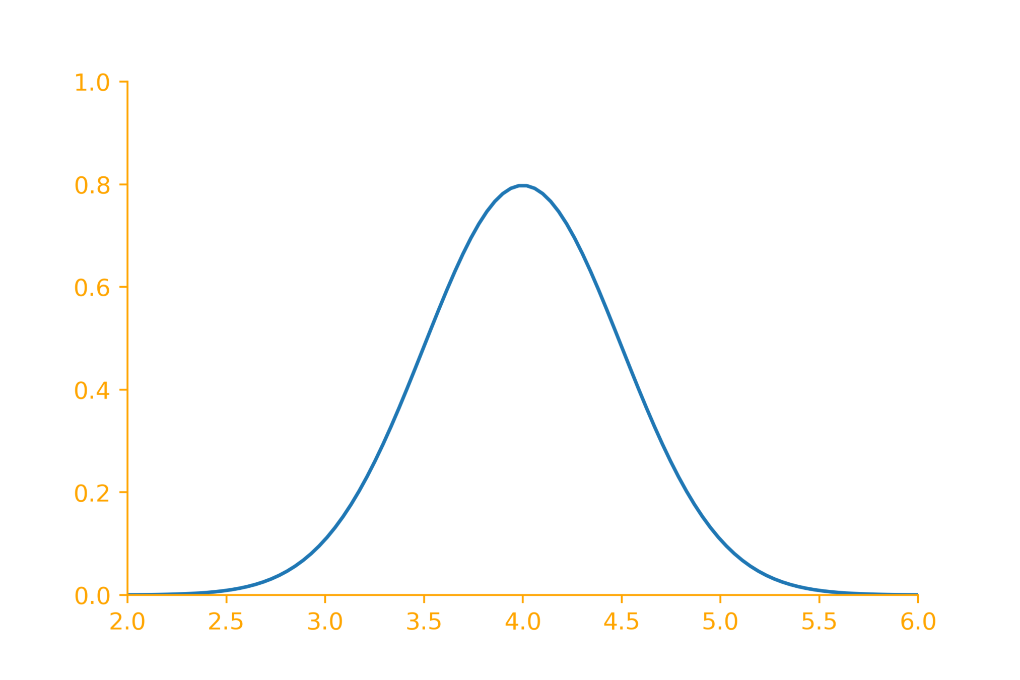
You have developed a new dialog system and done a user study. You claim that the average rating given by the users is greater than 4 on a scale of 1 to 5. How do you prove this to your critiques?
\mu \leq 4
\mu > 4
Null hypothesis
Alternative hypothesis
status quo*
a bold claim
* there is no surprise in this
How do you test your hypothesis?
Ask n users to use and rate your system
Compute mean rating
Now what?
You have developed a new dialog system and done a user study. You claim that the average rating given by the users is greater than 4 on a scale of 1 to 5. How do you prove this to your critiques?
\mu \leq 4
\mu > 4
Null hypothesis
Alternative hypothesis
Not always! because we know that the sample means follow a distribution
status quo*
a bold claim
Suppose the mean rating of the sample is 4.3, should the critiques accept your claim?
It is possible to get a sample whose mean is 4.3 even if the population mean is 4 or less?
How likely is it to get such a mean if the true population mean is 4?
(figuring this out is the goal of this lecture)
If it is very unlikely then reject the null hypothesis
\leq
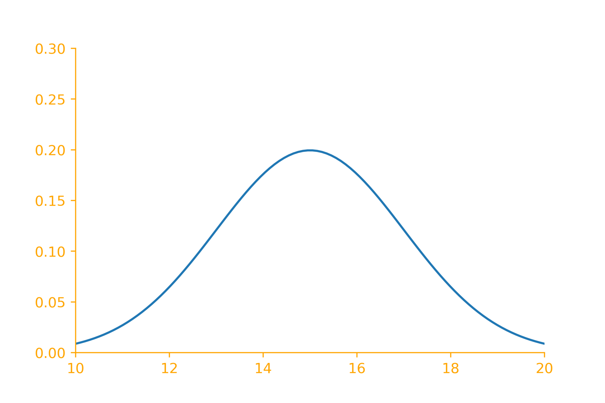
You have developed an AI powered fuel management system for SUVs. You claim that with this system, on average the SUV's mileage is at least 15 km/litre?
\mu \leq 15
\mu > 15
Null hypothesis
Alternative hypothesis
status quo*
a bold claim
* there is no surprise in this
How do you test your hypothesis?
Install your system in n SUVs (or install in one SUV and test it n times)
Compute mean mileage
Now what?
You have developed an AI powered fuel management system for SUVs. You claim that with this system, on average the SUV's mileage is at least 15 km/litre?
\mu \leq 15
\mu > 15
Null hypothesis
Alternative hypothesis
status quo*
a bold claim
Not always! because we know that the sample means follow a distribution
Suppose the mean mileage of the sample is 19 km/litre, should the an investor believe your claims?
It is possible to get a sample whose mean is 17 even if the population mean is 15 or less?
How likely is it to get such a mean if the true population mean is 15?
(figuring this out is the goal of this lecture)
If it is very unlikely then reject the null hypothesis
\leq
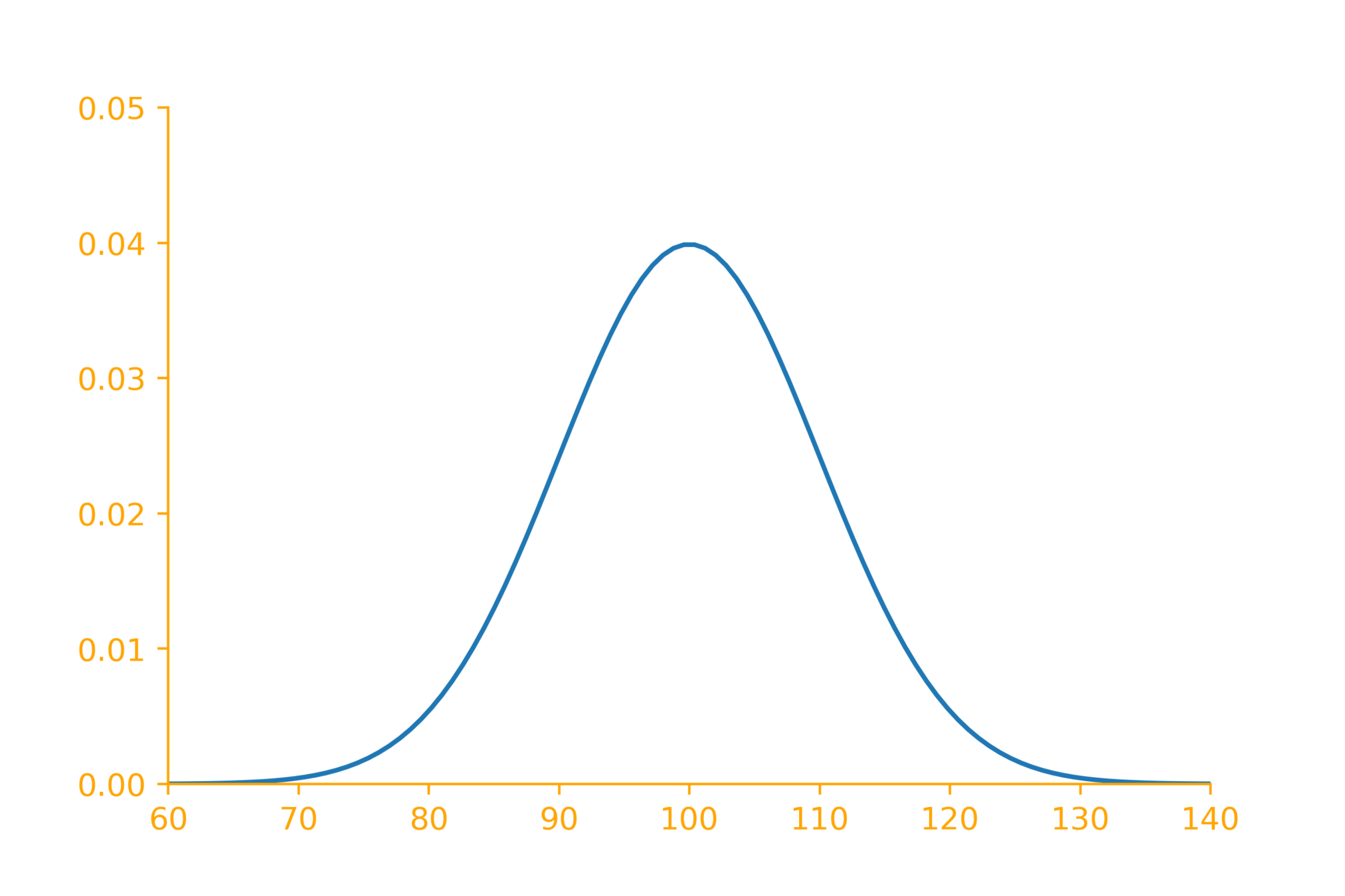
You have developed a new image classification system and claim that on average it takes less than 100 ms to classify one image . How do you convince your reviewers about this claim?
\mu \geq 100
\mu < 100
Null hypothesis
Alternative hypothesis
*
a bold claim
* there is no surprise in this
How do you test your hypothesis?
Feed n images to your system
Compute the mean classification time
Now what?
You have developed a new image classification system and claim that on average it takes less than 100 ms to classify one image . How do you convince your reviewers about this claim?
\mu \geq 100
\mu < 100
Null hypothesis
Alternative hypothesis
*
a bold claim
Not always! because we know that the sample means follow a distribution
Suppose the mean classification time is 95 ms, should the reviewers believe your claims?
It is possible to get a sample whose mean is 95 even if the population mean is 100 or more?
How likely is it to get such a mean if the true population mean is 100?
(figuring this out is the goal of this lecture)
If it is very unlikely then reject the null hypothesis
\geq
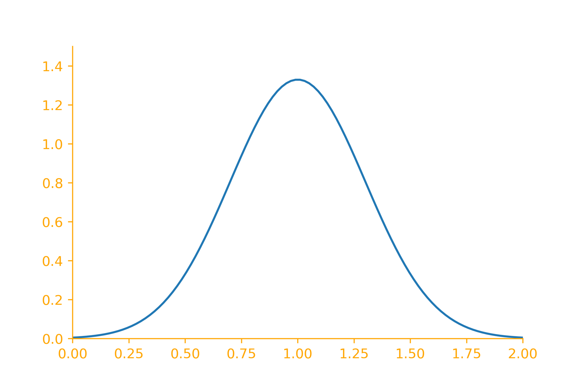
You have developed a new machine translation system and claim that on average it takes less than 1 MB memory per sentence . How do you convince your reviewers about this claim?
\mu \geq 1
\mu < 1
Null hypothesis
Alternative hypothesis
*
a bold claim
* there is no surprise in this
How do you test your hypothesis?
Feed n sentences to your system
Compute the mean memory per sentence
Now what?
You have developed a new machine translation system and claim that on average it takes less than 1 MB memory per sentence . How do you convince your reviewers about this claim?
\mu \geq 1
\mu < 1
Null hypothesis
Alternative hypothesis
*
a bold claim
Not always! because we know that the sample means follow a distribution
Suppose the mean memory is 0.95 MB, should the reviewers believe your claims?
It is possible to get a sample whose mean is 0,95 even if the population mean is 1 or more?
How likely is it to get such a mean if the true population mean is 1?
(figuring this out is the goal of this lecture)
If it is very unlikely then reject the null hypothesis
\geq
Three cases
Null hypothesis
Alternative hypothesis
H_0:
H_1:
\mu = 200
\mu \neq 200
H_0:
H_1:
\mu = 3
\mu \neq 3
H_0:
H_1:
\mu \leq 4
\mu > 4
H_0:
H_1:
\mu \leq 15
\mu > 15
H_0:
H_1:
\mu \geq 100
\mu < 100
H_0:
H_1:
\mu \geq 1
\mu < 1
In general,
H_0:
H_1:
\mu = \mu_0
\mu \neq \mu_0
H_0:
H_1:
\mu \leq \mu_0
\mu > \mu_0
H_0:
H_1:
\mu \geq \mu_0
\mu < \mu_0
Three cases
H_0:
H_1:
\mu = \mu_0
\mu \neq \mu_0
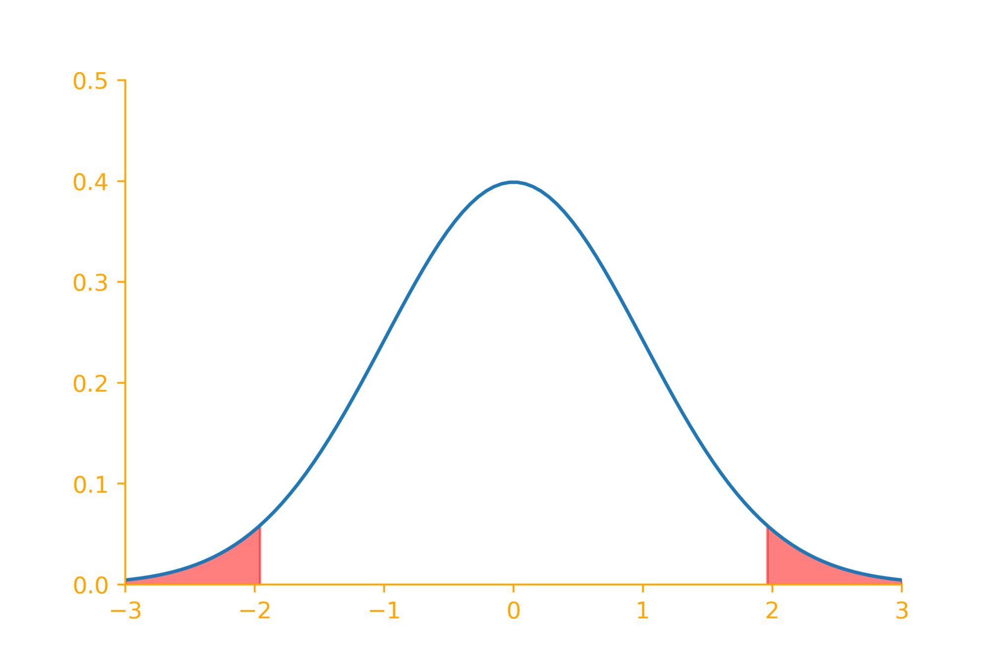
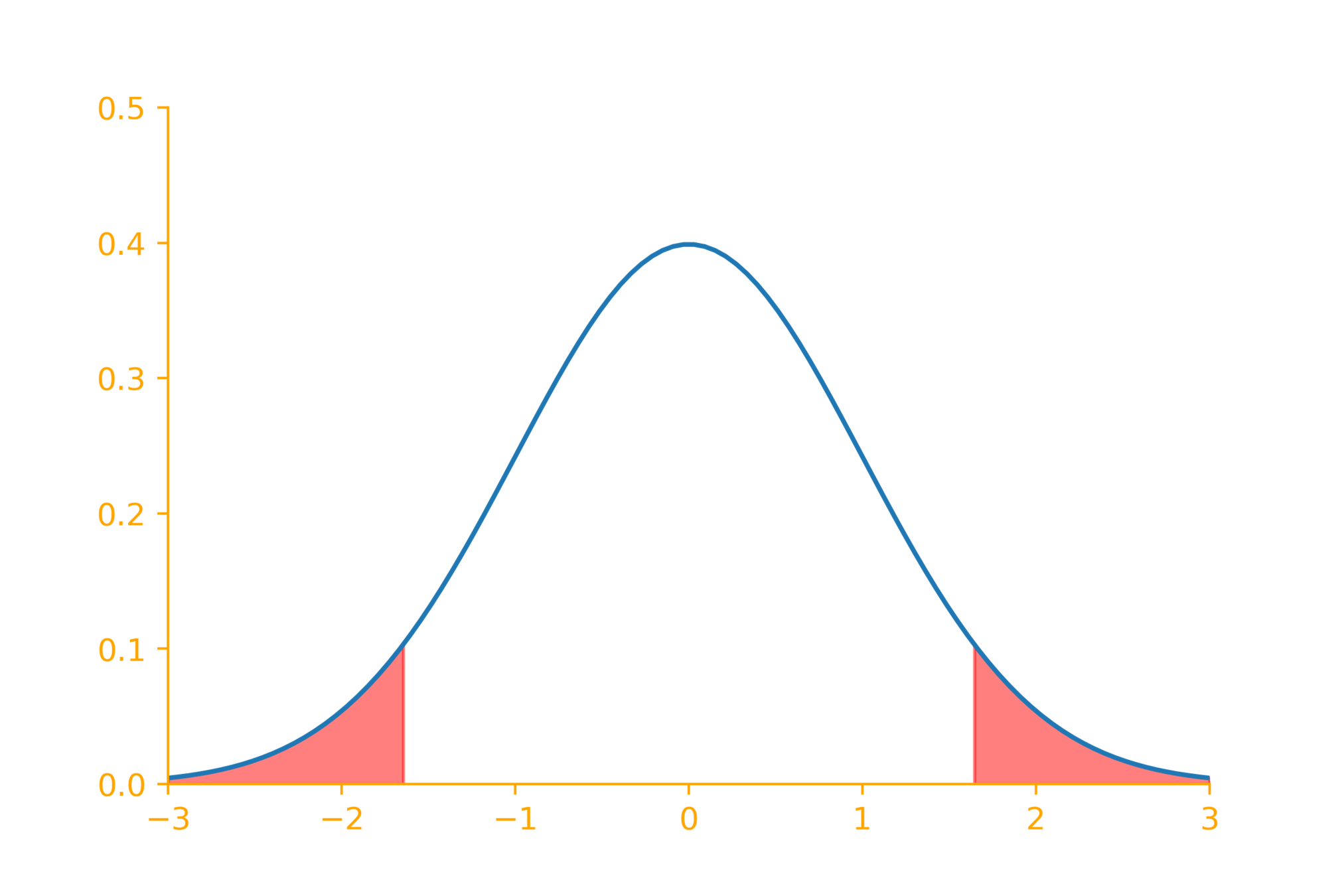
If the null hypothesis was indeed true then there is a very little chance of observing a sample whose mean is in the red zone
(< 5\%~chance)
So reject the null hypothesis!
\underbrace{~~~~~~~~~}_{2.5\%}
\underbrace{~~~~~~~~~}_{2.5\%}
H_0:
H_1:
\mu \leq \mu_0
\mu > \mu_0
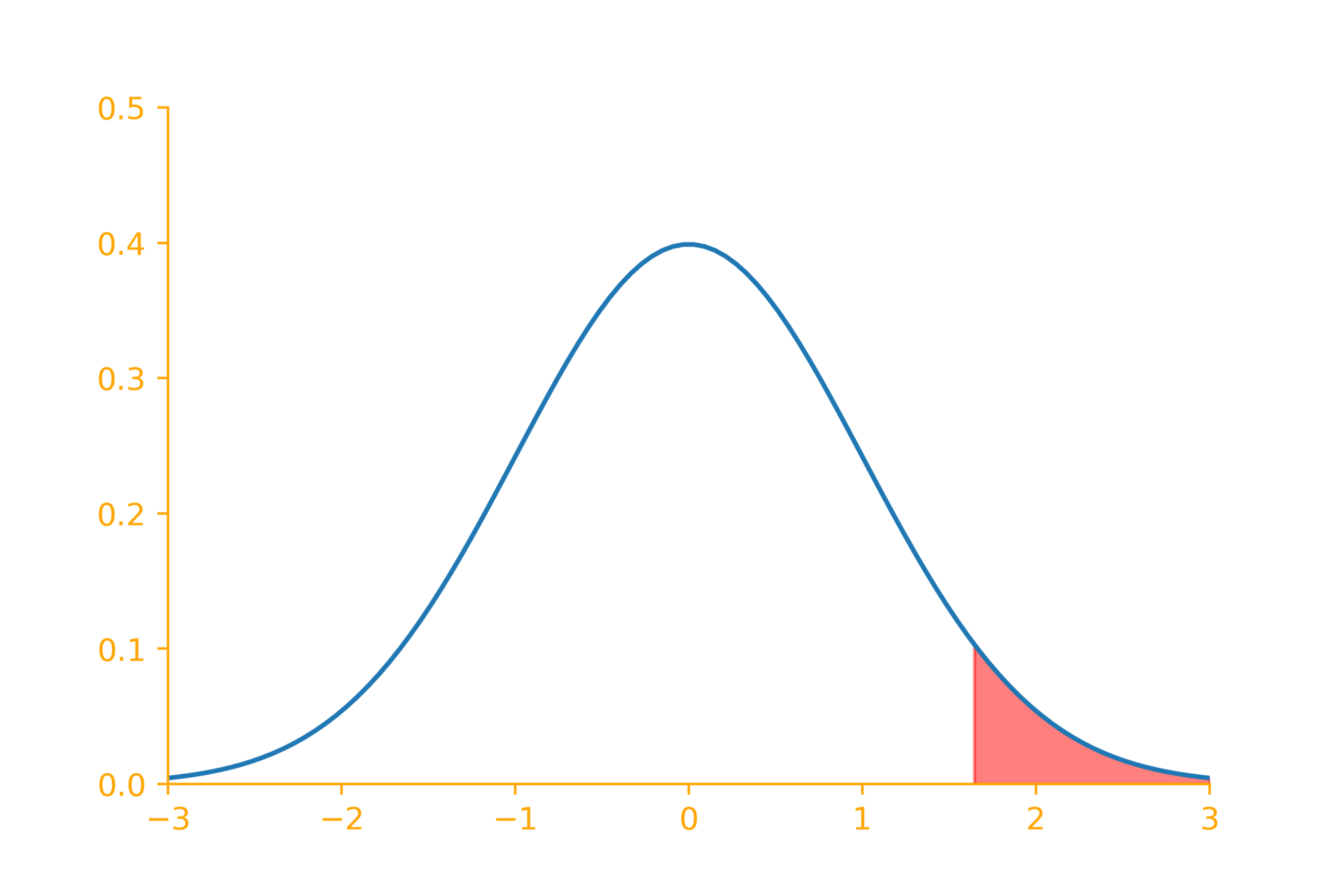
\underbrace{~~~~~~~~~~~~}_{5\%}

H_0:
H_1:
\mu \geq \mu_0
\mu < \mu_0
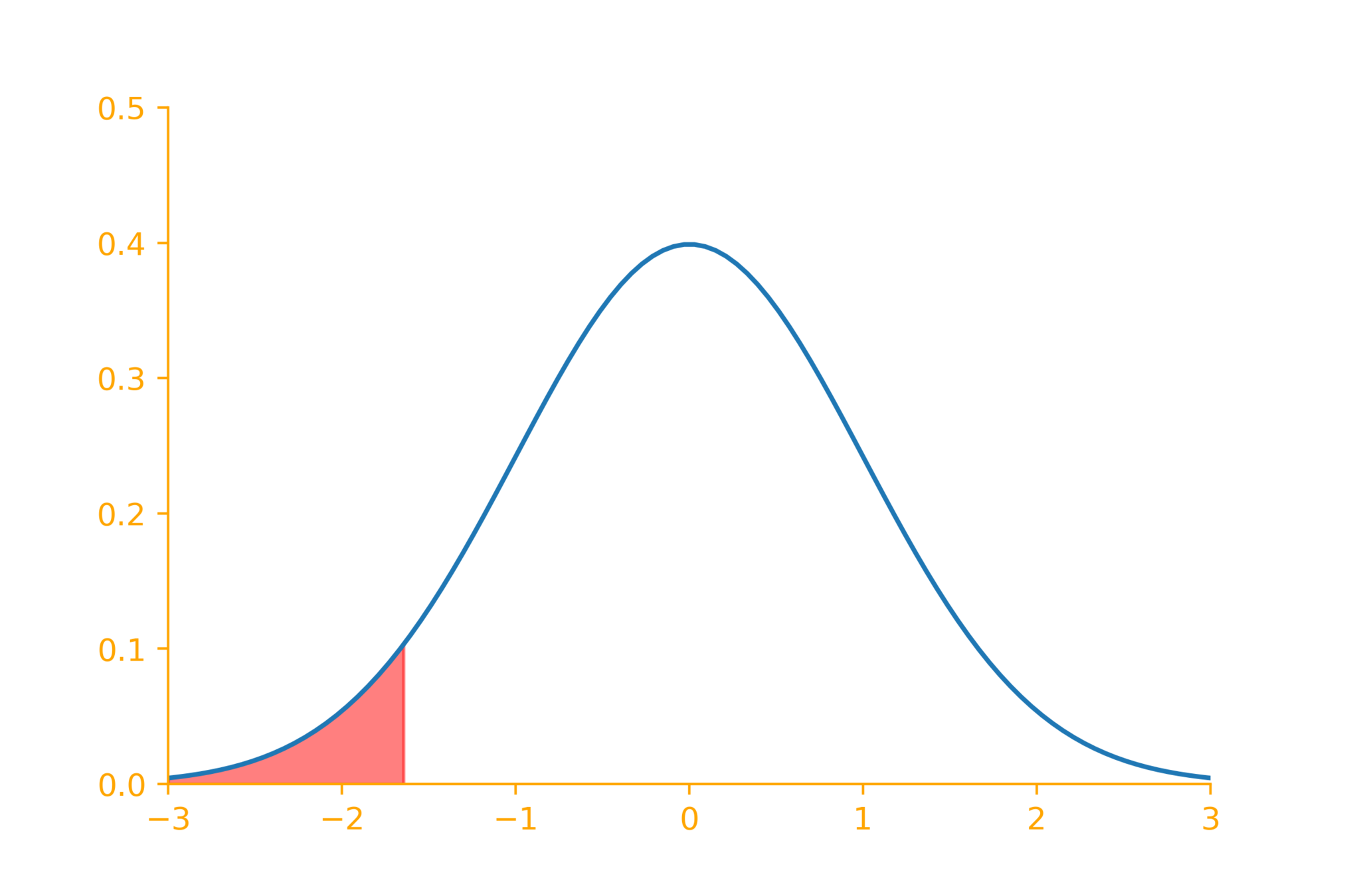
\underbrace{~~~~~~~~~~~~}_{5\%}
Terminology

Rejection region: If the sample mean lies in this region we will reject the null hypothesis
\underbrace{~~~~~~~~~}_{2.5\%}
\underbrace{~~~~~~~~~}_{2.5\%}
Significance level : Decides the critical region - typical values are 0.01 (1%), 0.05 (5%), 0.1(10%)
\alpha
-value : The probability that a sample mean would be greater than the mean computed from this sample
p
mean computed from the current sample
* In all the above definitions replace sample mean by any test statistic
Mapping to standard normal


weight of chips
mileage
classification time
All are normally distributed random variables but with different means and variances
In each case we are interested in knowing whether the sample mean lies in the critical region
Easier to just convert each of them to a standard normal random variable
\(Z = \dfrac{\overline{X} - \mu_0}{\sigma/\sqrt{n}}\)
\mu_0 = 200
\mu_0 = 15
\mu_0 = 100
number of samples

\sqrt{variance}
standard deviation
Mapping to standard normal


weight of chips
mileage
classification time
\mu_0 = 200
\mu_0 = 15
\mu_0 = 100
\(Z = \dfrac{\overline{X} - \mu_0}{\sigma/\sqrt{n}}\)
z
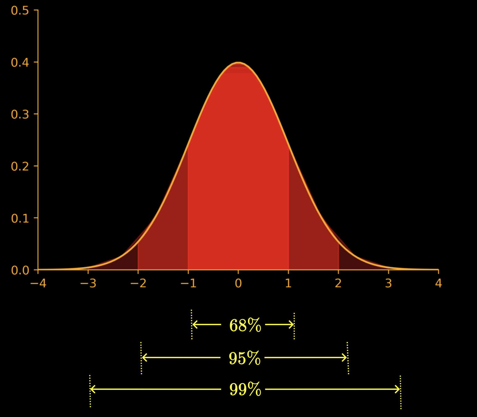
The regions are already well defined for the standard normal distribution
Critical regions
\alpha = 0.05
\(z = \dfrac{\overline{x} - \mu_0}{\sigma/\sqrt{n}}\)

+1.96
-1.96
Reject null hypothesis if
H_0:
H_1:
\mu = \mu_0
\mu \neq \mu_0
|z| > 1.96

H_0:
H_1:
\mu \leq \mu_0
\mu > \mu_0
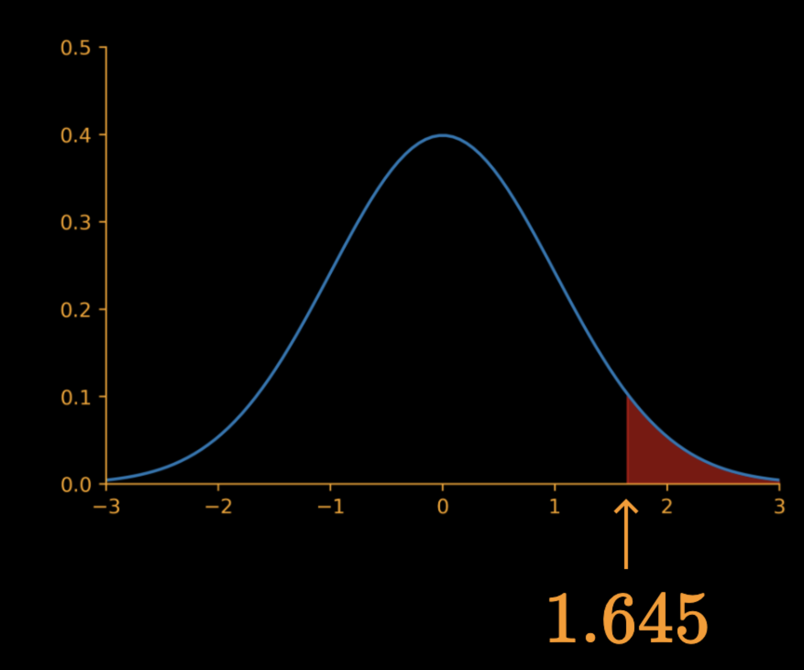
1.645
Reject null hypothesis if
z > 1.645

H_0:
H_1:
\mu \geq \mu_0
\mu < \mu_0
-1.645
Reject null hypothesis if
z < -1.645
Critical regions
\alpha = 0.1
\(z = \dfrac{\overline{x} - \mu_0}{\sigma/\sqrt{n}}\)
+1.645
-1.645
Reject null hypothesis if
H_0:
H_1:
\mu = \mu_0
\mu \neq \mu_0
|z| > 1.645
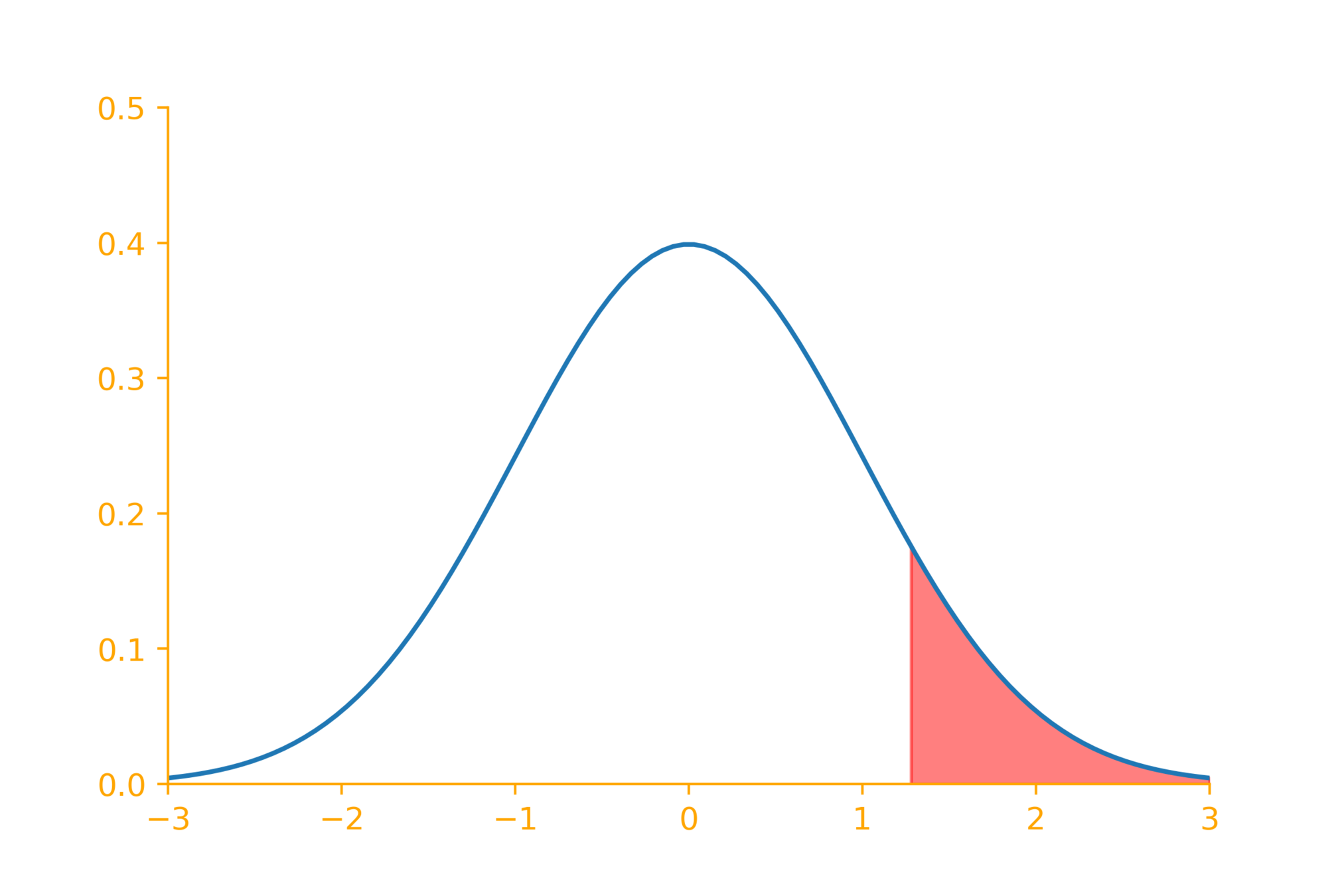
H_0:
H_1:
\mu \leq \mu_0
\mu > \mu_0
1.28
Reject null hypothesis if
z > 1.28
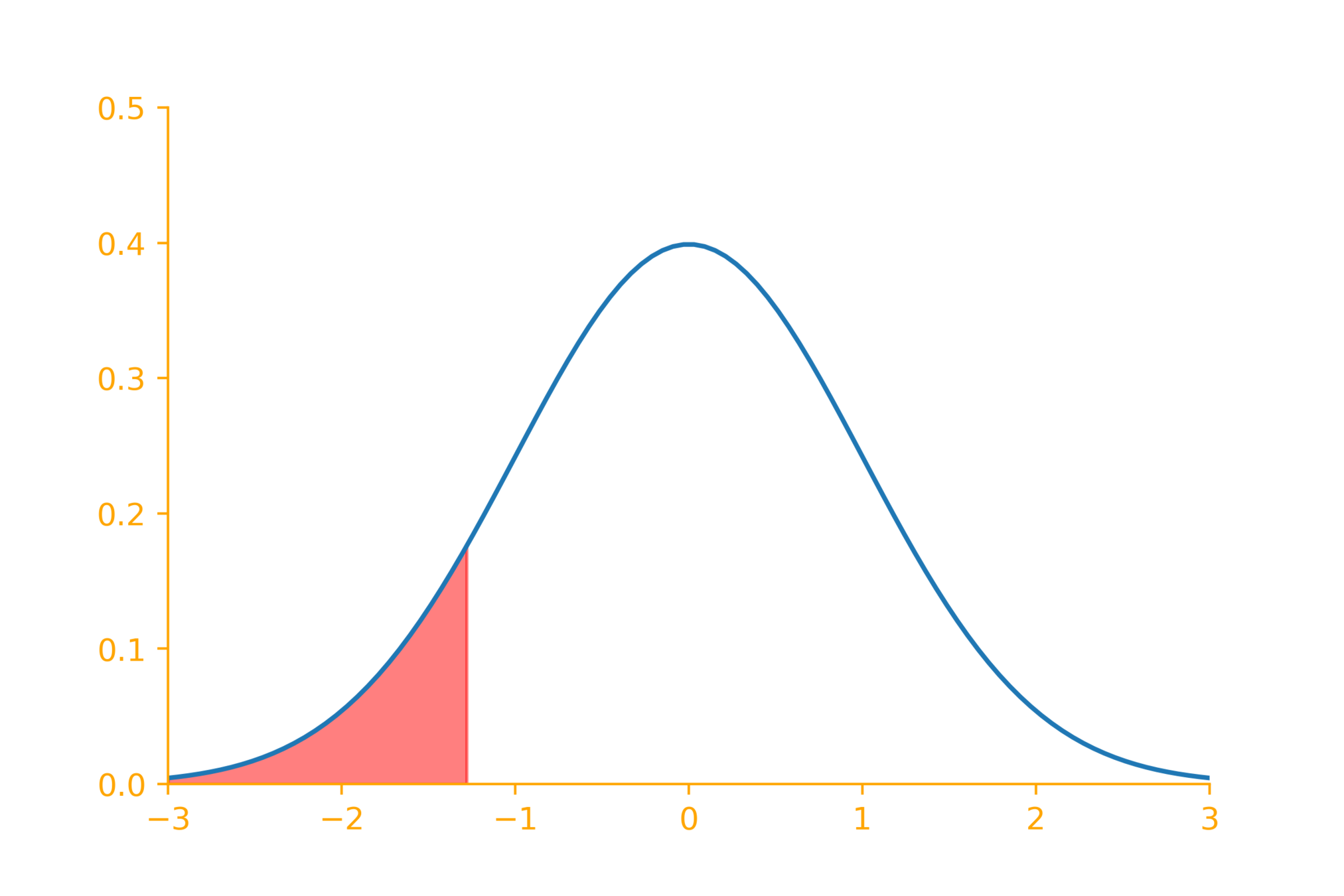
H_0:
H_1:
\mu \geq \mu_0
\mu < \mu_0
-1.28
Reject null hypothesis if
z < -1.28
Critical regions
\alpha = 0.01
\(z = \dfrac{\overline{x} - \mu_0}{\sigma/\sqrt{n}}\)
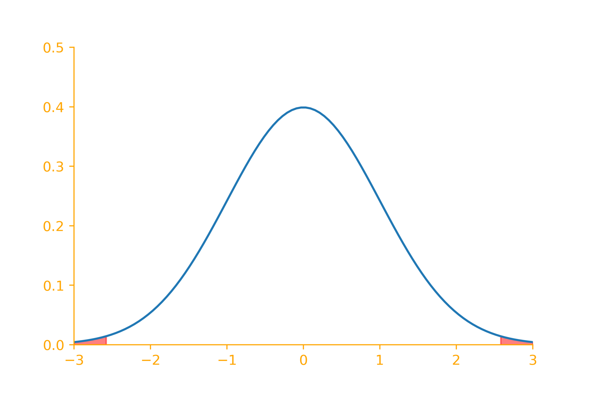
+2.58
-2.58
Reject null hypothesis if
H_0:
H_1:
\mu = \mu_0
\mu \neq \mu_0
|z| > 2.58
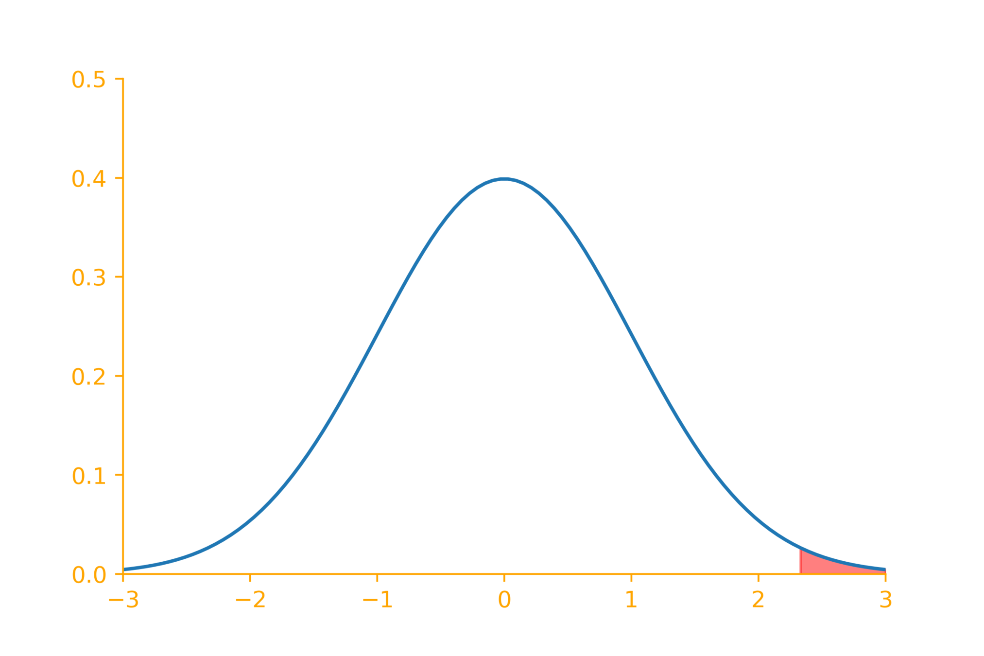
H_0:
H_1:
\mu \leq \mu_0
\mu > \mu_0
2.33
Reject null hypothesis if
z > 2.33
H_0:
H_1:
\mu \geq \mu_0
\mu < \mu_0
-2.33
Reject null hypothesis if
z < -2.33
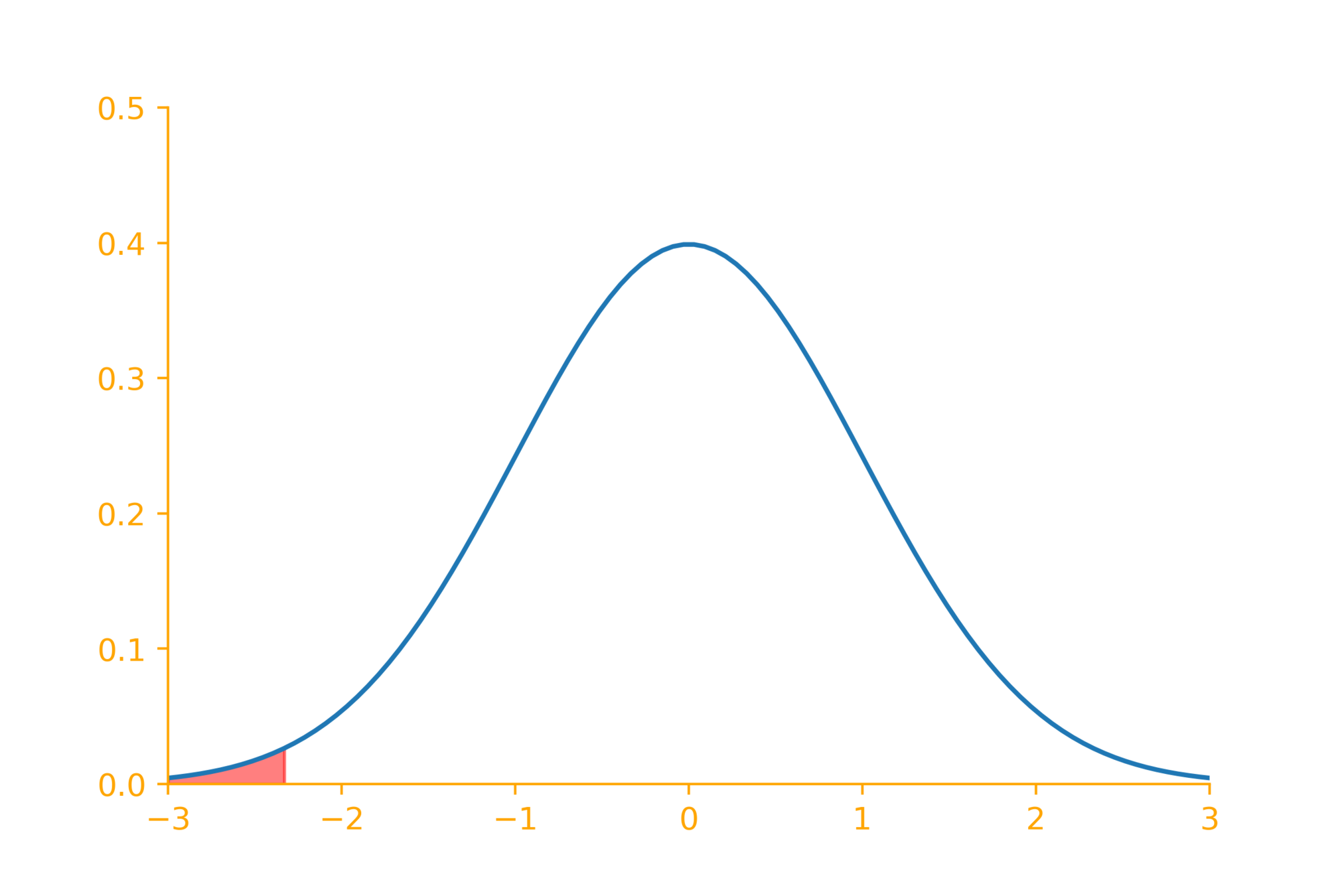
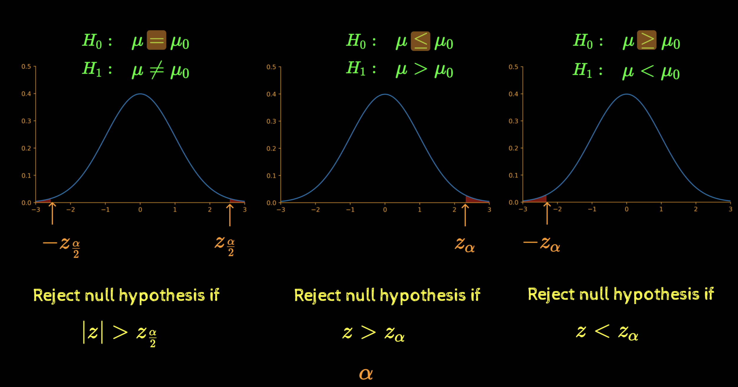
Critical regions
\alpha
\(Z = \dfrac{\overline{X} - \mu_0}{\sigma/\sqrt{n}}\)
z_{\frac{\alpha}{2}}
-z_{\frac{\alpha}{2}}
Reject null hypothesis if
H_0:
H_1:
\mu = \mu_0
\mu \neq \mu_0
|z| > z_{\frac{\alpha}{2}}

H_0:
H_1:
\mu \leq \mu_0
\mu > \mu_0
z_\alpha
Reject null hypothesis if
z > z_{\alpha}

H_0:
H_1:
\mu \geq \mu_0
\mu < \mu_0
-z_\alpha
Reject null hypothesis if
z < z_{\alpha}

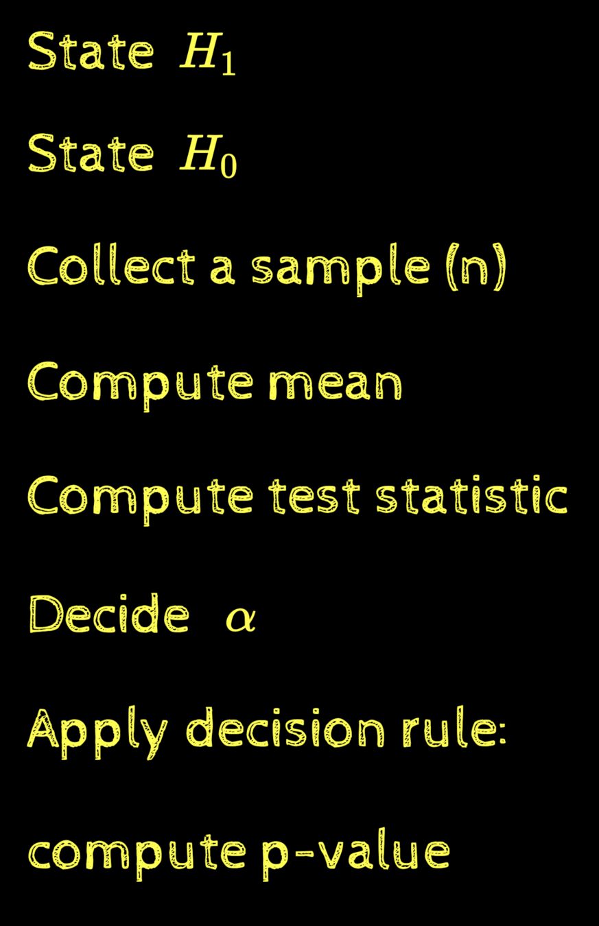
The steps in a hypothesis test
H_1
State
a bold claim
H_0
State
the opposite of
H_1
Collect a sample (n)
the larger the better
Compute mean
say,
\overline{x}
Compute test statistic
\(z = \dfrac{\overline{x} - \mu_0}{\sigma/\sqrt{n}}\)
Decide
\alpha
\alpha=0.01, 0.05, 0.1
Apply decision rule:
|z| > z_{\frac{\alpha}{2}}
z > z_\alpha
z < -z_\alpha
H_1:
\mu \neq \mu_0
H_1:
\mu > \mu_0
H_1:
\mu < \mu_0
Variance: Known or Unknown
z = \dfrac{\overline{x} - \mu_0}{\sigma/\sqrt{n}}
Case 1: Population variance is known
Case 2: Population variance is unknown
\sqrt{variance}
We will now revisit our case studies for both the situations (variance known, variance unknown)
A company selling chips claims that each packet has 200 grams of chips (as mentioned on the label). You are sceptic of their claims and believe that on average each packet does not contain 200 grams of chips. Based on past data you know that the standard deviation is 10 grams. How will you prove your claim?
H_0: \mu = 200
H_1: \mu \neq 200
H_1
State
H_0
State
Collect a sample (n)
Compute mean
Compute test statistic
Decide
\alpha
Apply decision rule:
[193, 212, 174, 200, 195, 195, 194, 198, 181, 203]
\overline{x} = 194.5
z = \dfrac{\overline{x} - \mu_0}{\sigma/\sqrt{n}} = \frac{194.5 - 200}{10/\sqrt{10}} = -1.739
say, \alpha = 0.05
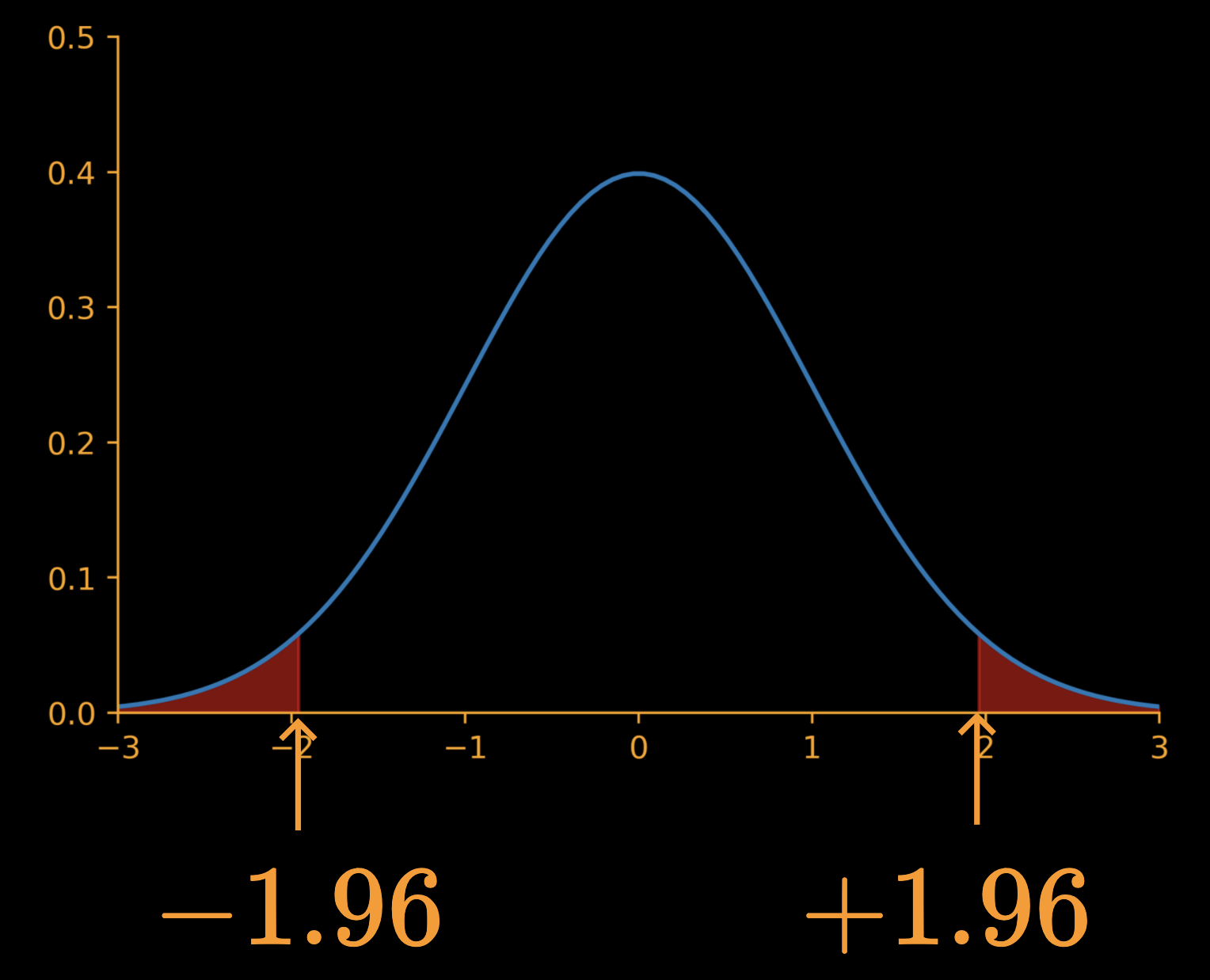
(reject~H_0~if~|z| > z_{\frac{\alpha}{2}})
|-1.739| < 1.96
Can't reject the null hypothesis
compute p-value
1.739
-1.739
p~value = P(|z| > \overline{x}) = 0.082
A company manufacturing ball bearing claims that the average radius of the ball bearings is 3 mm? Your company purchases these ball bearings and has asked you to verify this claim. Based on past data you know that the standard deviation is 0.1 mm. How will you go about verifying this?
H_0: \mu = 3
H_1: \mu \neq 3
H_1
State
H_0
State
Collect a sample (n)
Compute mean
Compute test statistic
Decide
\alpha
Apply decision rule:
[2.99, 2.99, 2.70, 2.92, 2.88, 2.92, 2.82, 2.83, 3.06, 2.85]
\overline{x} = 2.896
z = \dfrac{\overline{x} - \mu_0}{\sigma/\sqrt{n}} = \frac{2.896 - 3.0}{0.1/\sqrt{10}} = -3.28
say, \alpha = 0.01
(reject~H_0~if~|z| > z_{\frac{\alpha}{2}})
|-3.28| > 2.58
Reject the null hypothesis
compute p-value
-3.28
p~value = P(|z| > \overline{x}) = 0.001
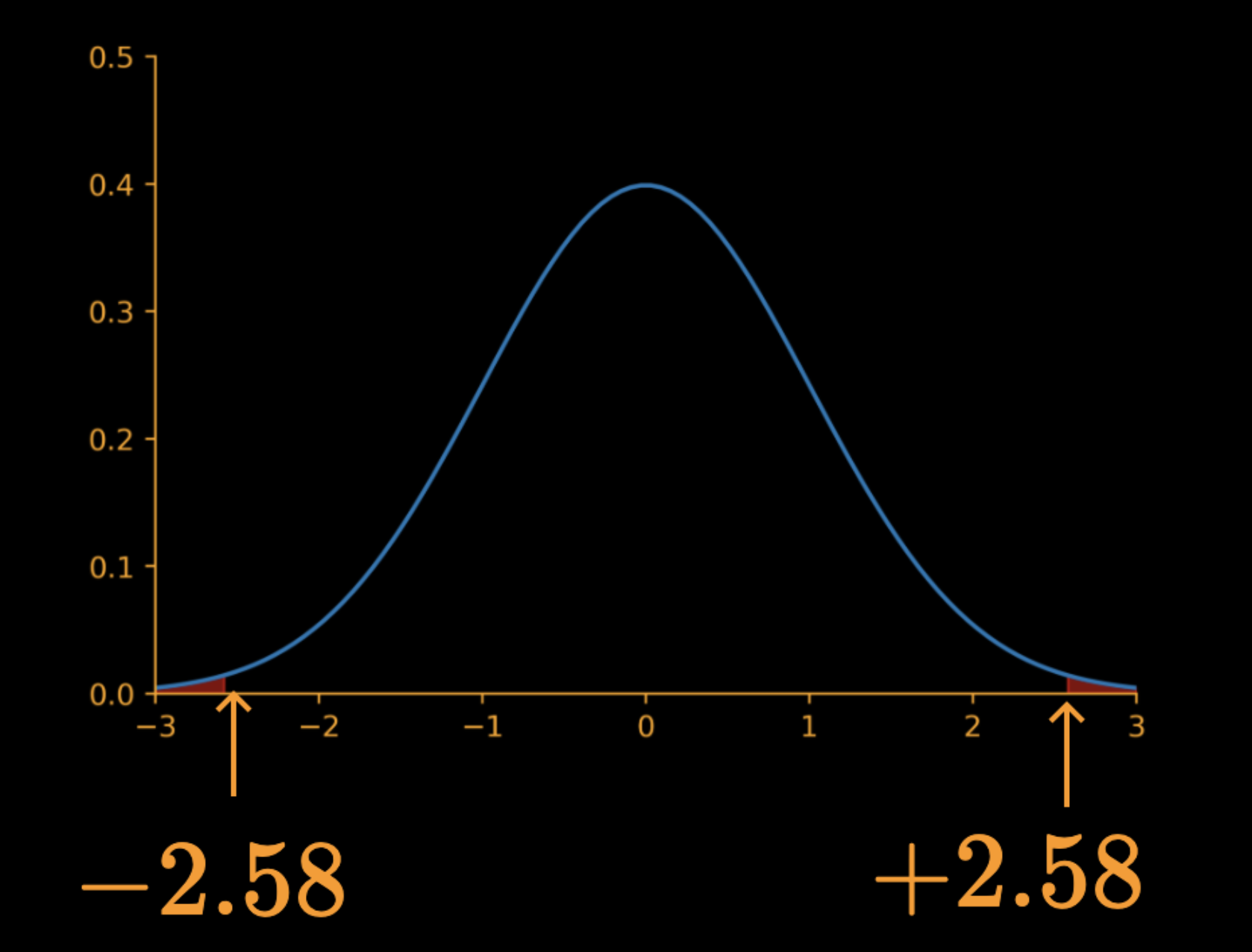
+3.28
Effect of
z = \dfrac{\overline{x} - \mu_0}{\sigma/\sqrt{n}} = \sqrt{n}\dfrac{\overline{x} - \mu_0}{\sigma}
If n is large we should expect sample mean to be closer to the population mean
Even small differences should lead to the null hypothesis getting rejected
The multiplication by square root n in the numerator ensures this
n,\sigma~and~\alpha
Effect of
z = \dfrac{\overline{x} - \mu_0}{\sigma/\sqrt{n}} = \sqrt{n}\dfrac{\overline{x} - \mu_0}{\sigma}
z = \dfrac{\overline{x} - \mu_0}{\sigma/\sqrt{n}} = \sqrt{10}\frac{194.5 - 200}{10} = -1.739

|-1.739| < 1.96
z = \dfrac{\overline{x} - \mu_0}{\sigma/\sqrt{n}} = \sqrt{100}\frac{194.5 - 200}{10} = -5.5
(reject~H_0~if~|z| > z_{\frac{\alpha}{2}})
|-5.5| > 1.96
z = \dfrac{\overline{x} - \mu_0}{\sigma/\sqrt{n}} = \sqrt{1000}\frac{199 - 200}{10} = -3.16
p~value = 0.082
p~value = 0.00001
|-3.16| > 1.96
p~value = 0.002
n,\sigma~and~\alpha
cannot reject
can reject
can reject
H_0
H_0
H_0
Effect of
z = \dfrac{\overline{x} - \mu_0}{\sigma/\sqrt{n}} = \sqrt{n}\dfrac{\overline{x} - \mu_0}{\sigma}
n,\sigma~and~\alpha
If is large we should expect lot of deviation in sample mean from one sample to another
So small differences should not lead to the null hypothesis getting rejected
The division by in the denominator ensures this
\sigma
\sigma
Effect of
z = \dfrac{\overline{x} - \mu_0}{\sigma/\sqrt{n}} = \sqrt{n}\dfrac{\overline{x} - \mu_0}{\sigma}
n,\sigma~and~\alpha
z = \dfrac{\overline{x} - \mu_0}{\sigma/\sqrt{n}} = \frac{2.896 - 3.0}{0.1/\sqrt{10}} = -3.28
|-3.28| > 2.58
Reject the null hypothesis

z = \dfrac{\overline{x} - \mu_0}{\sigma/\sqrt{n}} = \frac{2.896 - 3.0}{0.2/\sqrt{10}} = -1.64
(reject~H_0~if~|z| > z_{\frac{\alpha}{2}})
|-1.64| < 2.58
Cannot reject the null hypothesis
+1.645
-1.645


+1.96
-1.96
+2.58
-2.58

\alpha=0.1
\alpha=0.05
\alpha=0.01
Effect of
n,\sigma~and~\alpha
Higher the , stricter is the requirement for rejecting the null hypothesis
\alpha
+1.645
-1.645


+1.96
-1.96
+2.58
-2.58

\alpha=0.1
\alpha=0.05
\alpha=0.01
Effect of
n,\sigma~and~\alpha
z = \dfrac{\overline{x} - \mu_0}{\sigma/\sqrt{n}} = \frac{2.85 - 3.0}{0.2/\sqrt{10}} = -2.37
Reject the null hypothesis
Reject the null hypothesis
Cannot reject the null hypothesis
(reject~H_0~if~|z| > z_{\frac{\alpha}{2}})
Back to case studies
You have developed a new dialog system and done a user study. You claim that the average rating given by the users is greater than 4 on a scale of 1 to 5. How do you prove this to your critiques? (Based on past data you know that the standard deviation is 0.5 )
H_0: \mu \leq 4
H_1: \mu > 4
H_1
State
H_0
State
Collect a sample (n)
Compute mean
Compute test statistic
Decide
\alpha
Apply decision rule:
[4, 3, 5, 4, 5, 3, 5, 5, 4, 2, 4, 5, 5, 4, 4, 5, 4, 5, 4, 5]
\overline{x} = 4.25
z = \dfrac{\overline{x} - \mu_0}{\sigma/\sqrt{n}} = \frac{4.25 - 4}{0.5/\sqrt{20}} = 2.23
say, \alpha = 0.05
(reject~H_0~if~z > z_{\alpha})
2.23 > 1.645
Reject the null hypothesis
compute p-value
2.23
p~value = P(z > \overline{x}) = 0.012
You have developed AI powered fuel management system for SUVs. You claim that with this system, on average the SUV's mileage is at least 15 km/litre? (Based on past data you know that the standard deviation is 1 )
H_0: \mu \leq 15
H_1: \mu > 15
H_1
State
H_0
State
Collect a sample (n)
Compute mean
Compute test statistic
Decide
\alpha
Apply decision rule:
[14.08, 14.13, 15.65, 13.78, 16.26, 14.97, 15.36, 15.81, 14.53, 16.79, \\
15.78, 16.98, 13.23, 15.43, 15.46, 13.88, 14.31, 14.41, 15.76, 15.38]
\overline{x} = 15.1
z = \dfrac{\overline{x} - \mu_0}{\sigma/\sqrt{n}} = \frac{15.1 - 15}{1/\sqrt{20}} = 0.447
say, \alpha = 0.05
0.447 < 1.645
Cannot reject the null hypothesis
compute p-value
0.447
p~value = P(z > \overline{x}) = 0.327

(reject~H_0~if~z > z_{\alpha})
You have developed a new image classification system and claim that on average it takes less than 100 ms to classify one image . How do you convince your reviewers about this claim?(Based on past data you know that the standard deviation is 10 ms)
H_0: \mu \geq 100
H_1: \mu < 100
H_1
State
H_0
State
Collect a sample (n)
Compute mean
Compute test statistic
Decide
\alpha
Apply decision rule:
100~samples
\overline{x} = 97.5
z = \dfrac{\overline{x} - \mu_0}{\sigma/\sqrt{n}} = \frac{97.5 - 100}{10/\sqrt{100}} = -2.5
say, \alpha = 0.01
-2.5 < -2.33
Reject the null hypothesis
compute p-value
-2.5
p~value = P(z < \overline{x}) = 0.006
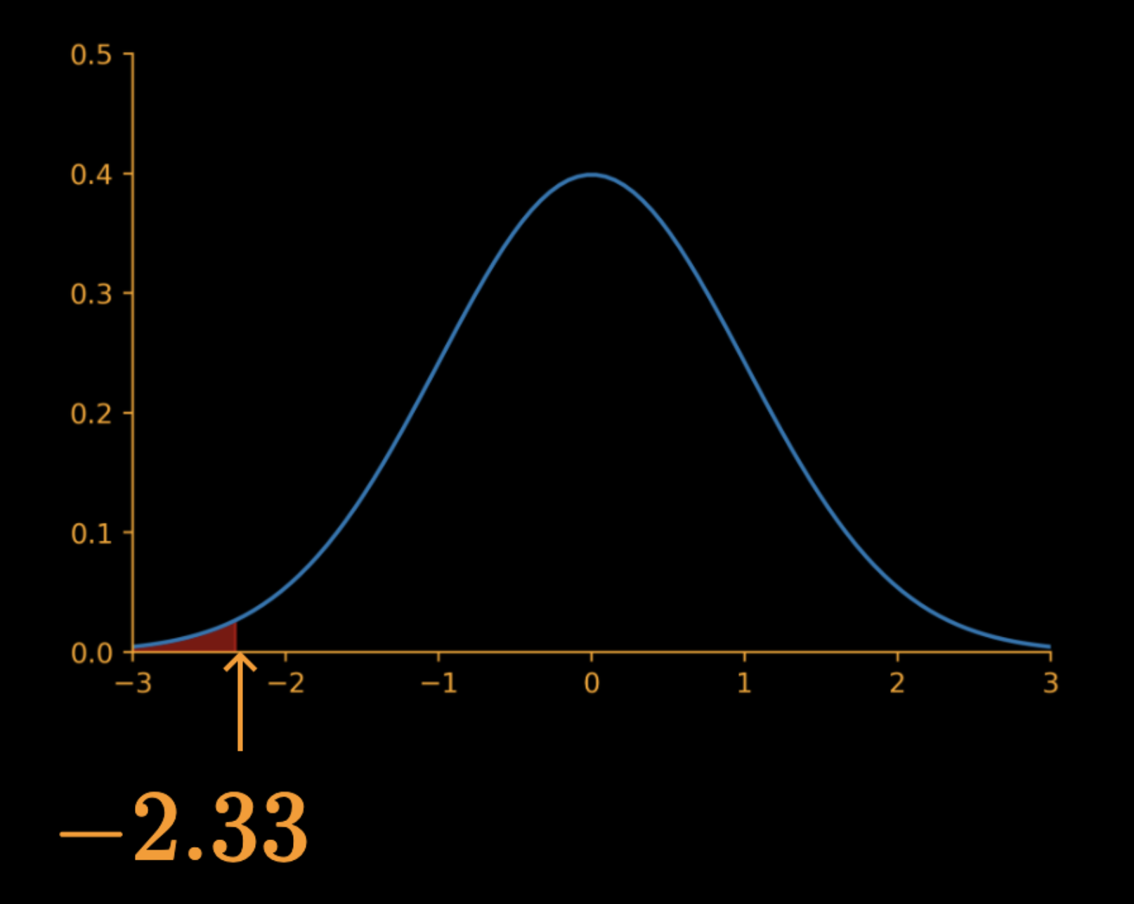
(reject~H_0~if~z < z_{\alpha})
You have developed a new machine translation system and claim that on average it takes less than 1 MB memory per sentence . How do you convince your reviewers about this claim? (Based on past data you know that the standard deviation is 0.1 MB)
H_0: \mu \geq 1
H_1: \mu < 1
H_1
State
H_0
State
Collect a sample (n)
Compute mean
Compute test statistic
Decide
\alpha
Apply decision rule:
100~samples
\overline{x} = 0.99
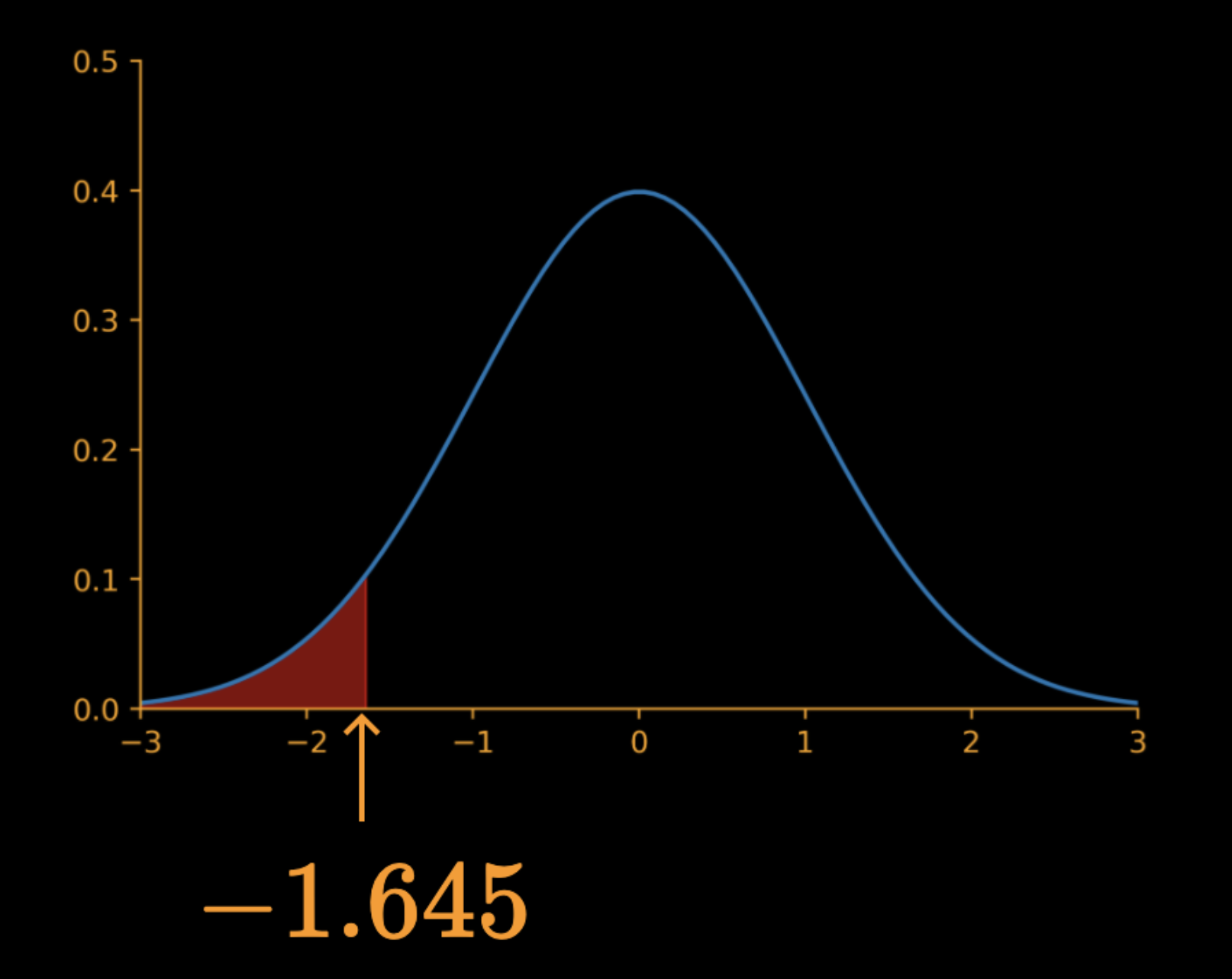
z = \dfrac{\overline{x} - \mu_0}{\sigma/\sqrt{n}} = \frac{0.99 - 1}{0.1/\sqrt{100}} = -1
say, \alpha = 0.05
-1 > -1.645
Cannot reject the null hypothesis
compute p-value
-1
p~value = P(z < \overline{x}) = 0.158
(reject~H_0~if~z < z_{\alpha})
Variance: Known or Unknown
z = \dfrac{\overline{x} - \mu_0}{\sigma/\sqrt{n}}
Case 1: Population variance is known
Case 2: Population variance is unknown
\sqrt{variance}
We will now revisit our case studies for both the situations (variance known, variance unknown)
Population variance is unknown
3 simple changes in our steps
t = \dfrac{\overline{x} - \mu_0}{s/\sqrt{n}}
|t| > t_{n-1,\frac{\alpha}{2}}
t > t_{n-1,\alpha}
t < t_{n-1,\alpha}
H_1
State
a bold claim
H_0
State
the opposite of
H_1
Collect a sample (n)
the larger the better
Compute mean and sd
say,
\overline{x}
s
and
Compute t test statistic
\(z = \dfrac{\overline{x} - \mu_0}{\sigma/\sqrt{n}}\)
Decide
\alpha
\alpha=0.01, 0.05, 0.1
Apply decision rule:
|z| > z_{\frac{\alpha}{2}}
z > z_\alpha
z < -z_\alpha
H_1:
\mu \neq \mu_0
H_1:
\mu > \mu_0
H_1:
\mu < \mu_0

z-test v/s t-test
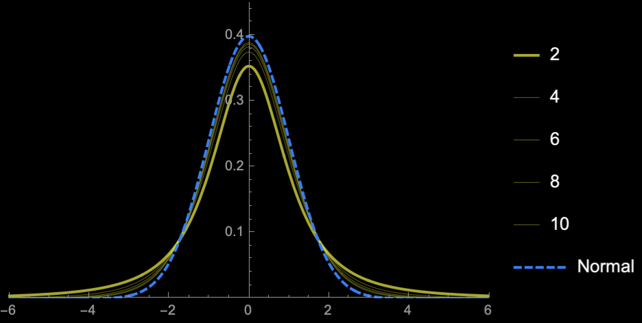
Student's \(t\)-distribution
\(\Rightarrow\) Higher uncertainty (Price of
not knowing \(\sigma\))
Normal distribution
(when variance is known)
(when variance is unknown)
\(z = \dfrac{\overline{x} - \mu_0}{\sigma/\sqrt{n}}\)
t = \dfrac{\overline{x} - \mu_0}{s/\sqrt{n}}
pop. std. dev.
sample std. dev.
|z| > z_{\frac{\alpha}{2}}
z > z_\alpha
z < -z_\alpha
H_1:
\mu \neq \mu_0
H_1:
\mu > \mu_0
H_1:
\mu < \mu_0
(depends on n-1)
H_1:
\mu \neq \mu_0
H_1:
\mu > \mu_0
H_1:
\mu < \mu_0
|t| > t_{n-1,\frac{\alpha}{2}}
t > t_{n-1,\alpha}
t < t_{n-1,\alpha}
no. of samples
You have developed a new dialog system and done a user study. You claim that the average rating given by the users is greater than 4 on a scale of 1 to 5. How do you prove this to your critiques? (Based on past data you know that the standard deviation is 0.5 )
H_0: \mu \leq 4
H_1: \mu > 4
H_1
State
H_0
State
Collect a sample (n)
Compute mean and sd
Compute t test statistic
Decide
\alpha
Apply decision rule:
[4, 3, 5, 4, 5, 3, 5, 5, 4, 2, 4, 5, 5, 4, 4, 5, 4, 5, 4, 5]
\overline{x} = 4.25
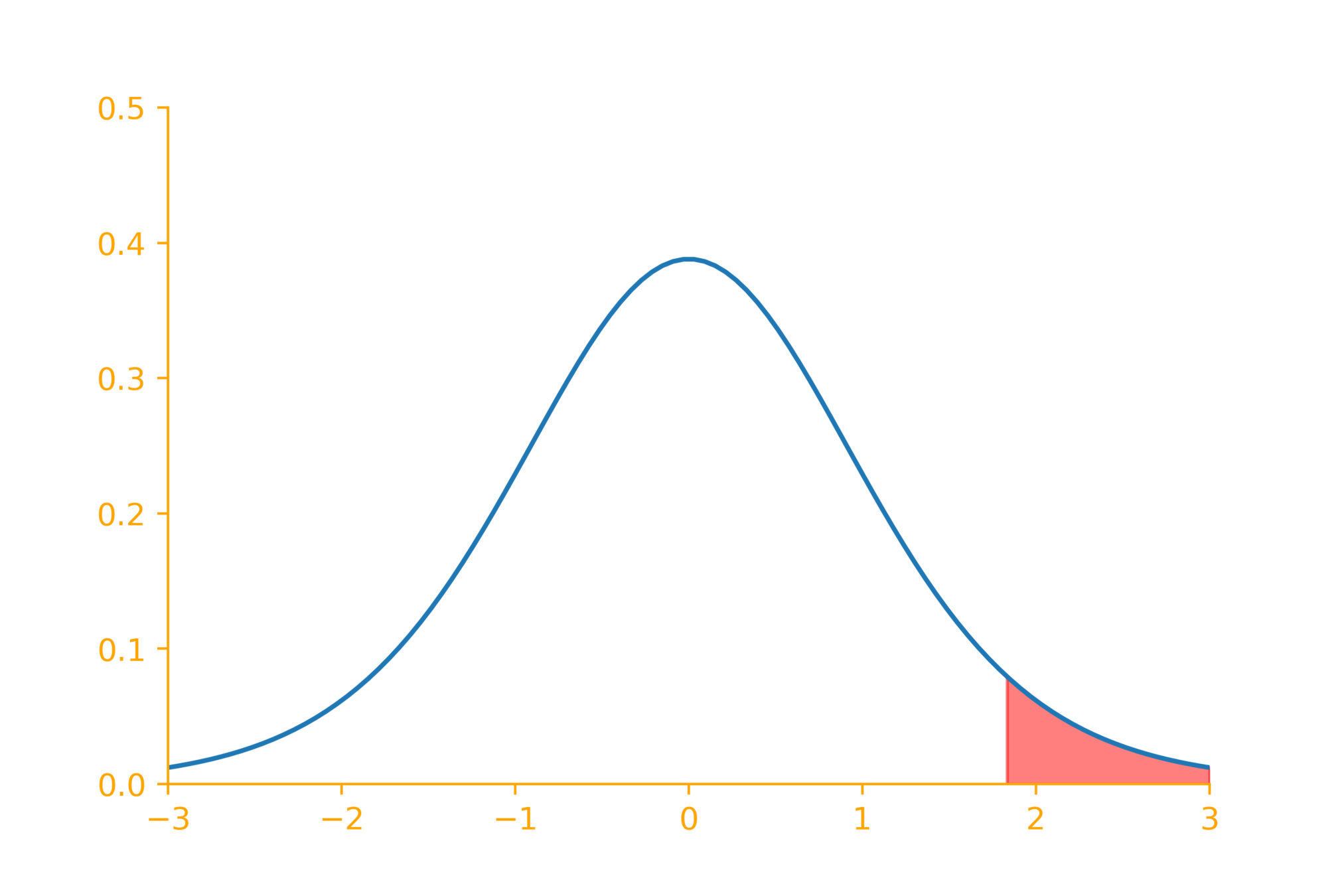
t = \dfrac{\overline{x} - \mu_0}{s/\sqrt{n}} = \frac{4.25 - 4}{0.85/\sqrt{20}} = 1.32
say, \alpha = 0.05
(reject~H_0~if~t > t_{n-1, \alpha})
1.32 < 1.73
Can't reject the null hypothesis
compute p-value
1.32
p~value = P(T > t) = 0.102
s = 0.85
1.73
df=9
A company selling chips claims that each packet has 200 grams of chips (as mentioned on the label). You are sceptic of their claims and believe that on average each packet does not contain 200 grams of chips. Based on past data you know that the standard deviation is 10 grams. How will you prove your claim?
H_0: \mu = 200
H_1: \mu \neq 200
H_1
State
H_0
State
Collect a sample (n)
Decide
\alpha
Apply decision rule:
[193, 212, 174, 200, 195, 195, 194, 198, 181, 203]
\overline{x} = 194.5
t = \dfrac{\overline{x} - \mu_0}{s/\sqrt{n}} = \frac{194.5 - 200}{10.7/\sqrt{10}} = -1.63
say, \alpha = 0.05
|-1.63| < 2.26
Can't reject the null hypothesis
compute p-value
1.63
-1.63
p~value = P(|T| > t) = 0.138
s = 10.7
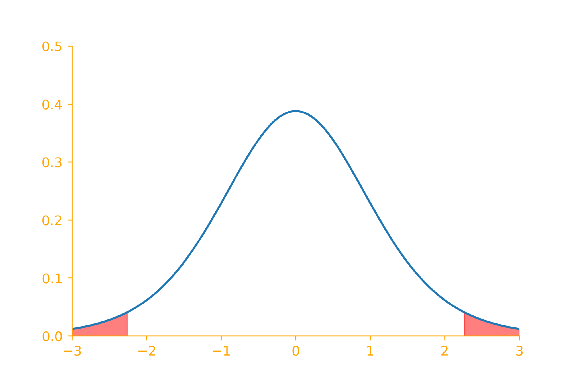
2.26
-2.26
Compute mean and sd
Compute t test statistic
(reject~H_0~if~t > t_{n-1, \alpha})
Hypothesis testing for proportion(p) instead of mean
You are teaching an online course and based on your internal surveys claim that 80% of your students like your course. A course review committee is skeptical about your claims abd wants to test them. How would they go about this
H_0: p \geq 0.8
H_1: p < 0.8
H_1
State
H_0
State
Hypothesis testing for proportion
z = \dfrac{\overline{p} - p_0}{\sqrt{p(1-p)}/\sqrt{n}}
H_1
State
a bold claim
H_0
State
the opposite of
H_1
Collect a sample (n)
the larger the better
Compute sample proportion
\overline{p}
Compute z test statistic
\(z = \dfrac{\overline{x} - \mu_0}{\sigma/\sqrt{n}}\)
Decide
\alpha
\alpha=0.01, 0.05, 0.1
Apply decision rule:
|z| > z_{\frac{\alpha}{2}}
z > z_\alpha
z < -z_\alpha
H_1:
\mu \neq \mu_0
H_1:
\mu > \mu_0
H_1:
\mu < \mu_0
You are teaching an online course and based on your internal surveys claim that 80% of your students like your course. A course review committee is skeptical about your claims abd wants to test them. How would they go about this
H_0: p \leq 0.8
H_1: p > 0.8
H_1
State
H_0
State
Collect a sample (n)
Decide
\alpha
Apply decision rule:
100~students~82~said~yes
\overline{p} = 0.82
say, \alpha = 0.05
0.5 > 1.645
cannot reject the null hypothesis
compute p-value
p~value = P(Z > z) = 0.308
Compute sample proportion
Compute z test statistic
(reject~H_0~if~z > z_{\alpha})
z = \dfrac{\overline{p} - p_0}{\sqrt{p(1-p)}/\sqrt{n}} = \dfrac{0.82 - 0.8}{\sqrt{0.8(1-0.8)}/\sqrt{100}} = 0.5
0.5

Type I and Type II errors
Type I and Type II errors
H_1:
(the courtroom analogy)
H_0:
Guilty
Not Guilty
prosecution's claim
default, status quo
(need convincing evidence)

less than 5% chance of seeing such damning evidence if the person was really not guilty
H_0
Reject
means that there is convincing evidence that the person is guilty
H_0
Cannot Reject
means that there is no convincing evidence that the person is guilty
(not the same as saying that there is convincing evidence that the person is not guilty)
Type I and Type II errors
H_1:
(the courtroom analogy)
H_0:
your claim
default, status quo
(need convincing evidence)

less than 5% chance of seeing such a sample if the status quo was really true
True Negative
False Positive
Real situation
Test Result
H_0~true
H_1~true
Don't~reject~H_0
Reject~H_0
False Negative
True Positive
Type I and Type II errors
H_1:
(the courtroom analogy)
H_0:
your claim
default, status quo
(need convincing evidence)

less than 5% chance of seeing such a sample if the status quo was really true
Type I error
Real situation
Test Result
H_0~true
H_1~true
Don't~reject~H_0
Reject~H_0
Type II error
Power of the test
\alpha
(1 - \alpha)
\beta
(1 - \beta)
Type I and Type II errors
(the courtroom analogy)

\mu_0
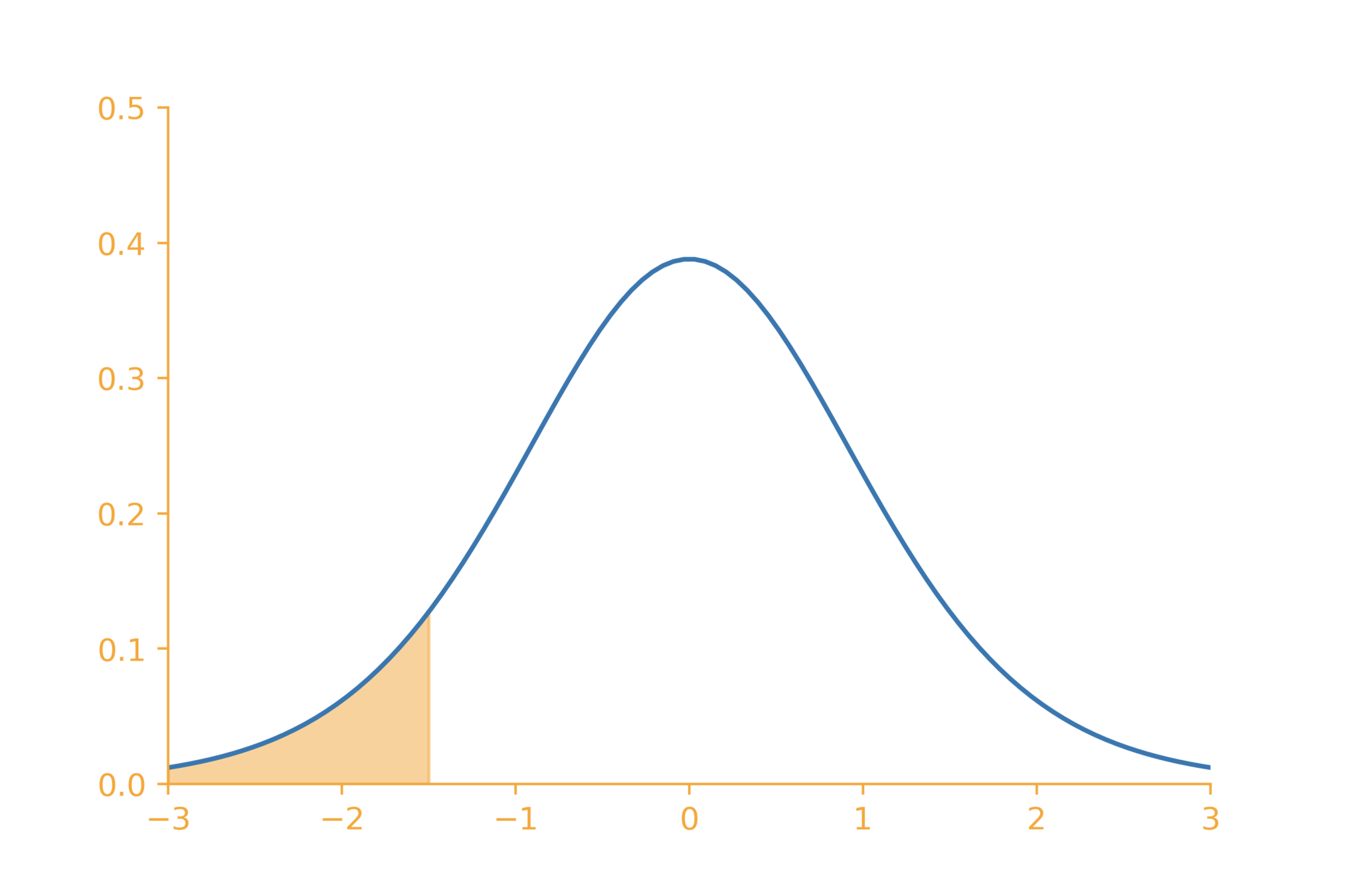
\mu_1
Guilty
Not Guilty
\underbrace{~~~~~\alpha~~~~~}
\underbrace{~~~~~~~~\beta~~~~~~}
\underbrace{~~~~~~~~~~~~~~~~~~~~~~~1 - \beta~~~~~~~~~~~~~~~~~~~~~~~}
Guilty will be set free
Guilty will be punished
innocent will be punished
Chi-Square test of independence
(case studies)
Is there a relationship between gender and preference of OS? (or does the preference of OS depend on the gender)
H_1
State
H_0
State
Collect a sample (n)
Compute sample frequencies
Compute test statistic
H_1:
H_0:
they are dependent
they are independent
| Male | Female | Total | |
|---|---|---|---|
| iOS | 25 | 40 | 65 |
| Windows | 60 | 70 | 130 |
| Linux | 20 | 30 | 50 |
| Total | 105 | 140 | 245 |
Observed frequencies (in sample)
| Male | Female | Total | |
|---|---|---|---|
| iOS | 27.85 | 37.15 | 65 |
| Windows | 55.70 | 74.30 | 130 |
| Linux | 21.50 | 28.50 | 50 |
| Total | 105 | 140 | 245 |
Expected frequencies (under null hyp.)
\frac{65}{245}
*105
\frac{65}{245}
*140
\chi^2
\chi^2 = \sum \frac{(o - e)^2}{e}
=\frac{(25-27.85)^2}{27.85} + \frac{(40-37.15)^2}{37.15} + \dots
=1.27
Is there a relationship between gender and preference of OS? (or does the preference of OS depend on the gender)
H_1
State
H_0
State
Collect a sample (n)
Decide
\alpha
Apply decision rule:
compute p-value
Compute sample frequencies
Compute test statistic
(reject~H_0~if~\chi^2 > \chi^2_{df,\alpha})
H_1:
H_0:
they are dependent
they are independent
\chi^2
\chi^2 = \sum \frac{(o - e)^2}{e}
=\frac{(25-27.85)^2}{27.85} + \frac{(40-37.15)^2}{37.15} + \dots
=1.27
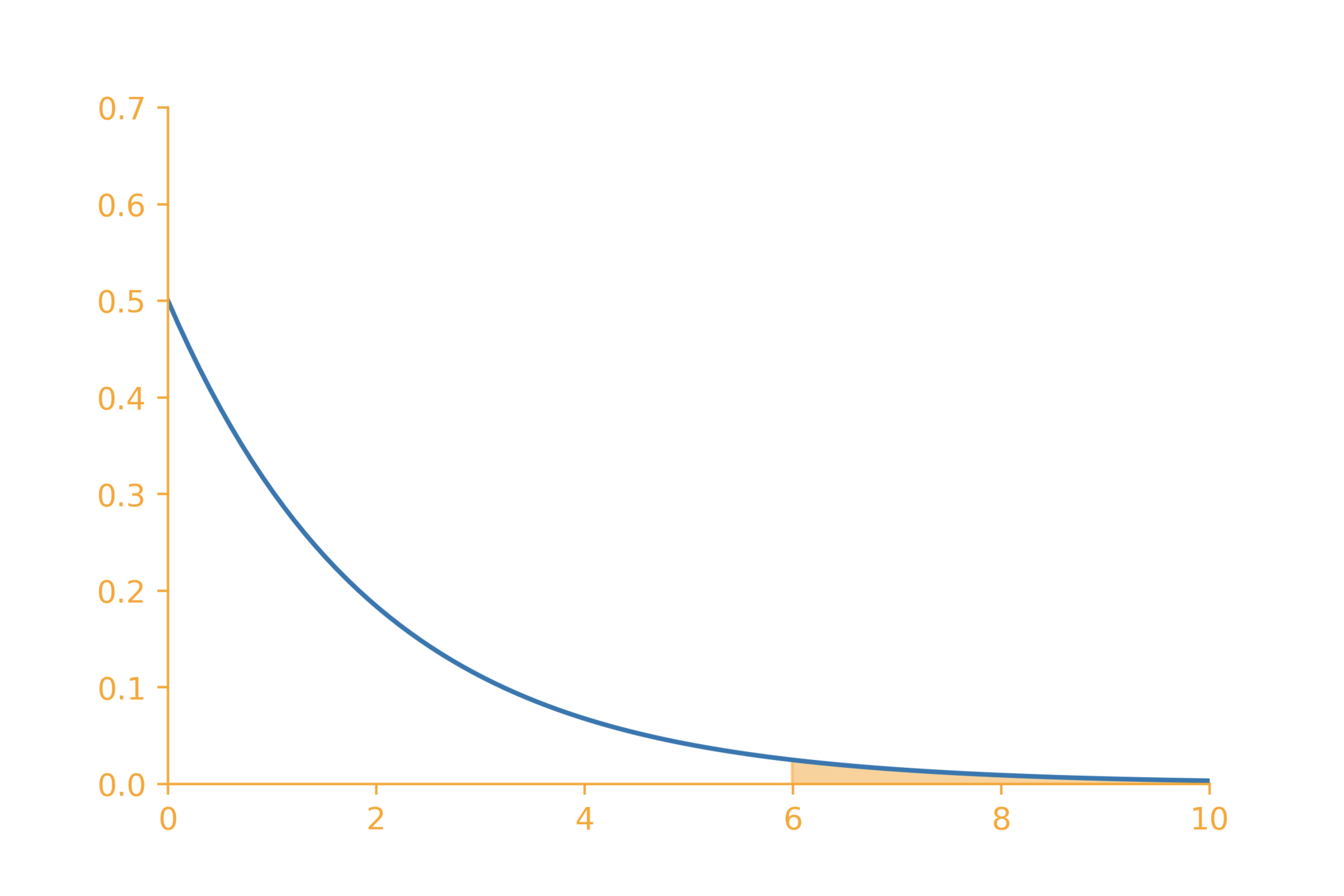
1.27
\chi^2_{~2,~0.05} = 5.99
df=2
cannot reject the null hypothesis
p~value = P(\chi^2_2 > 1.27) = 0.52
Degrees of Freedom
| Male | Female | Total | |
|---|---|---|---|
| iOS | 25 | 40 | 65 |
| Windows | 60 | 70 | 130 |
| Linux | 20 | 30 | 50 |
| Total | 105 | 140 | 245 |
Observed frequencies (in sample)
degrees of freedom = (rows - 1)(cols - 1)
| Married | Single | Divorced | Total | |
|---|---|---|---|---|
| Severe | 22 | 16 | 19 | 57 |
| Normal | 33 | 29 | 14 | 76 |
| Mild | 14 | 9 | 3 | 26 |
| Total | 69 | 54 | 36 | 159 |
Observed frequencies (in sample)
Is there a relationship between the marital status (married, single, divorced) of patients being treated for depression and the severity of their condition (severe, normal, mild) - S. Ross
State
State
Collect a sample (n)
Compute sample frequencies
Compute test statistic
H_1:
H_0:
they are dependent
they are independent
Expected frequencies (under null hyp.)
\frac{57}{159}
*69
\chi^2
\chi^2 = \sum \frac{(o - e)^2}{e}
=\frac{(22-24.75)^2}{24.75} + \frac{(16-19.35)^2}{19.35} + \dots
=6.83
| Married | Single | Divorced | Total | |
|---|---|---|---|---|
| Severe | 24.75 | 19.35 | 12.9 | 57 |
| Normal | 33.0 | 25.8 | 17.2 | 76 |
| Mild | 11.3 | 8.8 | 5.9 | 26 |
| Total | 69 | 54 | 36 | 159 |
Is there a relationship between the marital status (married, single, divorced) of patients being treated for depression and the severity of their condition (severe, normal, mild)
State
State
Collect a sample (n)
Decide
Apply decision rule:
compute p-value
Compute sample frequencies
Compute test statistic
(reject~H_0~if~\chi^2 > \chi^2_{df,\alpha})
H_1:
H_0:
they are dependent
they are independent
\chi^2
\chi^2 = \sum \frac{(o - e)^2}{e}
=\frac{(22-24.75)^2}{24.75} + \frac{(16-19.35)^2}{19.35} + \dots
=6.83
df = (rows - 1)(cols - 1) = 4
\alpha
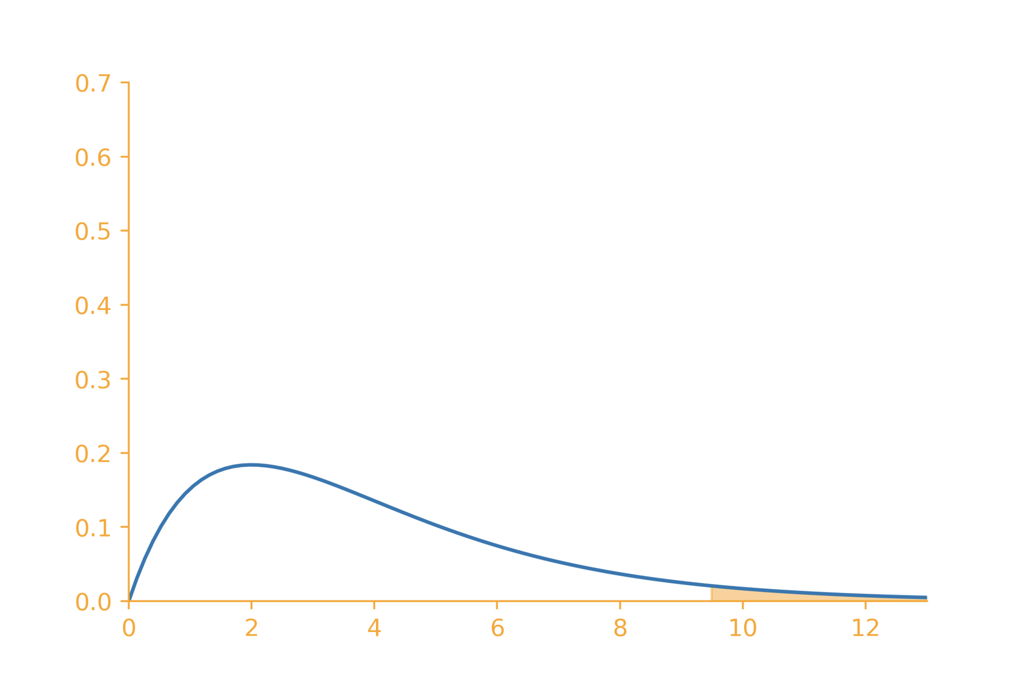
6.83
\chi^2_{~4,~0.05} = 9.49
df=4
cannot reject the null hypothesis
p~value = P(\chi^2_4 > 6.83) = 0.145
Summary
Mean
known variance
unknown variance
use normal dist.
use t dist. (df = n-1)
Proportion
use normal dist.
Independence
use Chi sq. dist.
H_1
State
H_0
State
Collect a sample (n)
Compute mean
Compute test statistic
Decide
\alpha