Our Roadmap


Given \(\mu, \sigma\)
\(E(\bar{X})\), \(Var(\bar{X})\)
Central Limit Theorem
Given \(\mu, \sigma\)
\(E(S)\), \(Var(S)\)
Chi Square Distribution
Given \(p\)
\(E(\hat{p})\), \(Var(\hat{p})\)
Our Roadmap


Given \(\mu, \sigma\)
\(E(\bar{X})\), \(Var(\bar{X})\)
Central Limit Theorem
Given \(\mu, \sigma\)
\(E(S)\), \(Var(S)\)
Chi Square Distribution
Given \(p\)
\(E(\hat{p})\), \(Var(\hat{p})\)
Notation
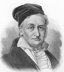
- C F Gauss
"We need notions, not notations"
Population Parameters - \(\mu, \sigma, p\)
Sample statistics - \(\bar{X}, S, \hat{p}\)
Statistics of sample statistics - \(\mathbb{E}[\bar{X}], \mathrm{sd}(\bar{X}), \mathrm{var}(\bar{X}), \\\mathbb{E}[S], \mathrm{sd}(S), \mathrm{var}(S), \\\mathbb{E}[\hat{p}], \mathrm{sd}(\hat{p}), \mathrm{var}(\hat{p})\)
Population Size - \(N\)
Size of each Sample - \(n\)
Number of samples - \(k\)
Items in a sample - \(X_1, X_2, \ldots, X_n\)
Computing \(\mathbb{E}[\bar{X}]\)
Given \(\mu, \sigma\)
What is your guess of \(\mathbb{E}[\bar{X}]\)?
What would you like it to be?
Close to \(\mu\)
Computing \(\mathbb{E}[\bar{X}]\)
Given \(\mu, \sigma\)
\(\mathbb{E}[\overline{X}]\)
\( = \mathbb{E}\left[\left(\frac{X_1+X_2 +\ldots + X_n}{n}\right)\right]\)
\( = \frac{1}{n}\mathbb{E}[X_1+X_2 +\ldots + X_n]\)
\( = \frac{1}{n}(\mathbb{E}[X_1]+\mathbb{E}[X_2] +\ldots + \mathbb{E}[X_n])\)
\( = \frac{1}{n}(\mu + \mu + \ldots + \mu)\)
\( = \mu\)
Linearity of expected value
Recall Random Sampling \(\Rightarrow X_1, X_2, \ldots X_n\) are independent
\(\mathbb{E}\) of sum of independent random vars is the sum of \(\mathbb{E}\) of individual variables
Recall each element of pop. is equally likely in samples
\(\mathbb{E}\) of any item in any sample is \(\mathbb{E}\) of any item in pop. = \(\mu\)
Computing \(\mathbb{E}[\bar{X}]\)
Given \(\mu, \sigma\)
\(\mathbb{E}[\overline{X}]\)
\( = \mu\)
Note that this is a "nice result"
Holds generally: independent of \(\sigma\), sample size \(n\)
\(\overline{X}\) is an unbiased estimate of \(\mu\)
Looks simple, but an important result
Computing \(\mathbb{E}[\bar{X}]\)
\(\mathbb{E}[\overline{X}]\)
\( = \mu\)
\(\overline{X}\) is an unbiased estimate of \(\mu\)
If we take any particular sample,
its \(\overline{X}\) can be less than or more than \(\mu\) but without any bias

Fair dice
\(\mu = 3.5\)
Systematic error
Individual samples vary,
but average of \(\overline{X} \approx 3.5\)

Computing \(\mathbb{E}[\bar{X}]\)
\(\mathbb{E}[\bar{X}]\)
\( = \mu\)

Fair dice
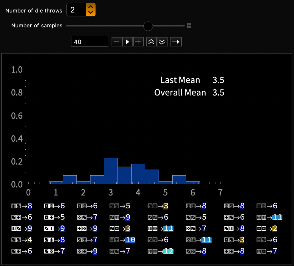
Vary sample size, number of samples
DEMO 1 of 2 - Discrete
Computing \(\mathbb{E}[\bar{X}]\)
\(\mathbb{E}[\bar{X}]\)
\( = \mu\)
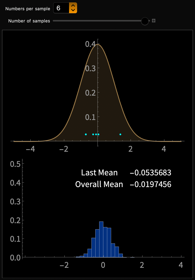
Sum of random variates from \(\mathcal{N}(0, 1)\)
DEMO 2 of 2 - Continuous

Our Roadmap


Given \(\mu, \sigma\)
\(E(\bar{X})\), \(Var(\bar{X})\)
Central Limit Theorem
Given \(\mu, \sigma\)
\(E(S)\), \(Var(S)\)
Chi Square Distribution
Given \(p\)
\(E(\hat{p})\), \(Var(\hat{p})\)
Our Roadmap


Given \(\mu, \sigma\)
\(E(\bar{X})\), \(Var(\bar{X})\)
Central Limit Theorem
Given \(\mu, \sigma\)
\(E(S)\), \(Var(S)\)
Chi Square Distribution
Given \(p\)
\(E(\hat{p})\), \(Var(\hat{p})\)
Computing \(\mathrm{var}(\bar{X})\)
Given \(\mu, \sigma\)
Compute \(\mathrm{var}(\overline{X})\)
What is your guess of \(\mathrm{var}(\overline{X})\)?
What would you like it to be?
Close to \(0\) would be nice
But definitely not more than \(\sigma^2\)
Computing \(\mathrm{var}(\bar{X})\)
Given \(\mu, \sigma\)
Compute \(\mathrm{var}(\bar{X})\)
Unlike the case of \(\mathbb{E}[\bar{X}]\), we will here build intuition before proof
Exercise 1
\(\bar{X}\) = Average of \(n\) throws of a die
Compute variance of \(\bar{X}\) of 1000 samples
Change \(n\) and recompute. Plot variance vs \(n\)
Computing \(\mathrm{var}(\bar{X})\)
Given \(\mu, \sigma\)
Compute \(\mathrm{var}(\bar{X})\)
Exercise 1
\(\bar{X}\) = Average of \(n\) throws of a die
Compute variance of \(\bar{X}\) over 1000 samples
Change \(n\) and recompute. Plot variance vs \(n\)
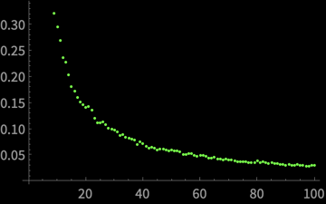
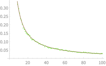
\(\mathrm{var}(\bar{X})\)
\(n\)
\(y \propto \frac{1}{x}\)
\(\mathrm{var}(\bar{X})\) falls inversely with \(n\)?
Computing \(\mathrm{var}(\bar{X})\)
Given \(\mu, \sigma\)
Compute \(\mathrm{var}(\bar{X})\)
Exercise 2
\(\bar{X}\) = Average of 10 numbers from \(\mathcal{N}(\mu, \sigma)\)
Compute variance of \(\bar{X}\) over 1000 samples
Change \(\mu\) and recompute. Plot variance vs \(\mu\)
Change \(\sigma\) and recompute. Plot variance vs \(\sigma\)
\(\mathrm{var}(\bar{X})\)
\(\mu\)
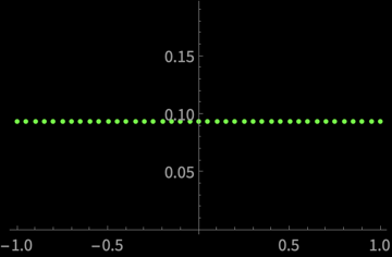
\(\mathrm{var}(\bar{X})\) is independent of \(\mu\)?
Computing \(\mathrm{var}(\bar{X})\)
Given \(\mu, \sigma\)
Compute \(\mathrm{var}(\bar{X})\)
Exercise 2
\(\bar{X}\) = Average of 10 samples from \(\mathcal{N}(\mu, \sigma)\)
Compute variance of \(\bar{X}\) over 1000 samples
Change \(\mu\) and recompute. Plot variance vs \(\mu\)
Change \(\sigma\) and recompute. Plot variance vs \(\sigma\)
\(\mathrm{var}(\bar{X})\)
\(\sigma\)
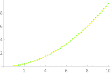
\(y \propto x^2\)
\(\mathrm{var}(\bar{X})\) is independent of \(\mu\)?
\(\mathrm{var}(\overline{X})\) scales as \(\sigma^2\)?
Computing \(\mathrm{var}(\bar{X})\)
Given \(\mu, \sigma\)
Compute \(\mathrm{var}(\bar{X})\)
\(\mathrm{var}(\bar{X})\) is independent of \(\mu\)?
\(\mathrm{var}(\overline{X})\) scales as \(\sigma^2\)?
\(\mathrm{var}(\bar{X})\)
\(=\frac{\sigma^2}{n}\)
Let's work towards a proof
Computing \(\mathrm{var}(\bar{X})\)
\(\mathrm{var}(\bar{X})\)
\(=\mathbb{E}[(\bar{X} - \mathbb{E}[\bar{X}])^2]\)
\(=\mathbb{E}[(\bar{X}^2 + \mathbb{E}[\bar{X}]^2 - 2\bar{X}\mathbb{E}[\bar{X}])\)
\(=\mathbb{E}[\bar{X}^2] + \mathbb{E}[\bar{X}]^2 - 2\mathbb{E}[\bar{X}]\mathbb{E}[\bar{X}]\)
\(=\mathbb{E}[\bar{X}^2] - \mathbb{E}[\bar{X}]^2 \)
A helpful reformulation of \(\mathrm{var}(\bar{X})\)
Computing \(\mathrm{var}(\bar{X})\)
\(\mathrm{var}(\bar{X})\)
\(=\mathbb{E}[\bar{X}^2] - \mathbb{E}[\bar{X}]^2 \)
\(\mathrm{var}(a\bar{X})\)
\(=\mathbb{E}[(a\bar{X})^2] - \mathbb{E}[(a\bar{X})]^2 \)
\(=a^2 (\mathbb{E}[\bar{X}^2] - \mathbb{E}[\bar{X}]^2) \)
\(=a^2 (\mathrm{var}(\bar{X})) \)
Computing \(\mathrm{var}(\bar{X})\)
\(\mathrm{var}(\bar{X})\)
\(=\mathbb{E}[\bar{X}^2] - \mathbb{E}[\bar{X}]^2 \)
\(\mathrm{var}(a\bar{X})\)
\(=a^2 (\mathrm{var}(\bar{X})) \)
\(\mathrm{var}(X_1 + X_2)\)
\(=\mathbb{E}[(X_1+X_2)^2] - \mathbb{E}[(X_1+X_2)]^2\)
\(=\mathbb{E}[X_1^2]+\mathbb{E}[X_2^2] + 2\mathbb{E}[X_1X_2]- \mathbb{E}[X_1]^2-\mathbb{E}[X_2]^2- 2\mathbb{E}[X_1]\mathbb{E}[X_2]\)
\(=\mathbb{E}[X_1^2] - \mathbb{E}[X_1]^2 + \mathbb{E}[X_2^2] - \mathbb{E}[X_2]^2\)
\(=\mathrm{var}(X_1) + \mathrm{var}(X_2)\)
Computing \(\mathrm{var}(\bar{X})\)
\(\mathrm{var}(\bar{X})\)
\(=\mathbb{E}[\bar{X}^2] - \mathbb{E}[\bar{X}]^2 \)
\(\mathrm{var}(a\bar{X})\)
\(=a^2 (\mathrm{var}(\bar{X})) \)
\(\mathrm{var}(X_1 + X_2)\)
\(=\mathrm{var}(X_1) + \mathrm{var}(X_2)\)
\(\mathrm{var}(\bar{X})\)
\(=\frac{1}{n^2}\mathrm{var}(X_1 + X_2 + \ldots + X_n) \)
\(=\mathrm{var}(\frac{X_1 + X_2 + \ldots + X_n}{n}) \)
\(=\frac{1}{n^2}(\mathrm{var}(X_1) + \mathrm{var}(X_2) + \ldots + \mathrm{var}(X_n) )\)
\(=\frac{1}{n^2}(\sigma^2 + \sigma^2 + \ldots + \sigma^2)\)
\(=\frac{\sigma^2}{n}\)
Computing \(\mathrm{var}(\bar{X})\)
\(\mathrm{var}(\bar{X})\)
\(\mathrm{sd}(\bar{X})\)
\(=\frac{\sigma^2}{n}\)
Implications
\(\bar{X}\) is an unbiased estimate. But it varies from sample to sample with \(\mathrm{sd} = \frac{\sigma}{\sqrt{n}}\)
To half \(\mathrm{sd}\) need to quadruple \(n\)
Cannot decrease \(\sigma\), can increase \(n\)
\(= \frac{\sigma}{\sqrt{n}}\)
Applied to Data Science


\(\overline{X_{income}}\)
\(\overline{X_{income}}\)
\(\overline{X_{income}}\)
\(\mu, \sigma\)
\(\overline{X_{income}}\) are unbiased estimates of \(\mu\)
But if they vary a lot from one sample to another, propose to increase sample size
Summary
Given population parameters \(\mu\) and \(\sigma\):

\(\mathbb{E}[\bar{X}] = \mu\)
\(\mathrm{var}(\bar{X}) = \frac{\sigma^2}{n}\)
Our Roadmap


Given \(\mu, \sigma\)
\(E(\bar{X})\), \(Var(\bar{X})\)
Central Limit Theorem
Given \(\mu, \sigma\)
\(E(S)\), \(Var(S)\)
Chi Square Distribution
Given \(p\)
\(E(\hat{p})\), \(Var(\hat{p})\)
Our Roadmap


Given \(\mu, \sigma\)
\(E(\bar{X})\), \(Var(\bar{X})\)
Central Limit Theorem
Given \(\mu, \sigma\)
\(E(S)\), \(Var(S)\)
Chi Square Distribution
Given \(p\)
\(E(\hat{p})\), \(Var(\hat{p})\)
Central Limit Theorem
\(\mathbb{E}[\bar{X}] = \mu\)
\(\mathrm{var}(\bar{X}) = \frac{\sigma^2}{n}\)
We know the mean and variance,
can we know more about the PDF of \(\bar{X}\)?
\(\overline{X} = \frac{1}{n}(X_1 + X_2 + \ldots + X_n)\)
Sum of \(n\) independent and identically distributed (iid) random variables
The Central Limit Theorem has something interesting to say about such sums
Central Limit Theorem
If \(X_1, X_2, \ldots, X_n\) are random samples from a population with mean \(\mu\) and finite standard deviation \(\sigma\), then the sum
\(X_1 + X_2 + \ldots + X_n\)
will converge to \(\mathcal{N}(n\mu, \sigma\sqrt{n})\) in the limiting condition of \(n\to \infty\)

Central Limit Theorem
If \(X_1, X_2, \ldots, X_n\) are random samples from a population with mean \(\mu\) and finite standard deviation \(\sigma\), then the sum
\(X_1 + X_2 + \ldots + X_n\)
will converge to \(\mathcal{N}(n\mu, \sigma\sqrt{n})\) in the limiting condition of \(n\to \infty\)

Awesome result!
Independent of the PDF of the population, the PDF of the sum of many samples tends to the normal distribution
Check that our derived results on \(\mathbb{E}(\overline{X})\) and \(\mathrm{sd}(\overline{X})\) remain true for large \(n\)
Exercise
Central Limit Theorem
Independent of the PDF of the population, the PDF of the sum of many samples tends to the normal distribution
Exercise
Plot the empirical distribution of sum of \(n\) iid samples from distribution \(\mathcal{D}\)
Do this for \(n = 10, 100, 1000, 10000\)
\(\mathcal{D}\) = Uniform, Binomial, Bimodal, Discrete
If \(X_1, X_2, \ldots, X_n\) are random samples from a population with mean \(\mu\) and finite standard deviation \(\sigma\), then the sum
\(X_1 + X_2 + \ldots + X_n\)
will converge to \(\mathcal{N}(n\mu, \sigma\sqrt{n})\) in the limiting condition of \(n\to \infty\)

Central Limit Theorem
If \(X_1, X_2, \ldots, X_n\) are random samples from a population with mean \(\mu\) and finite standard deviation \(\sigma\), then the sum
\(X_1 + X_2 + \ldots + X_n\)
will converge to \(\mathcal{N}(n\mu, \sigma\sqrt{n})\) in the limiting condition of \(n\to \infty\)

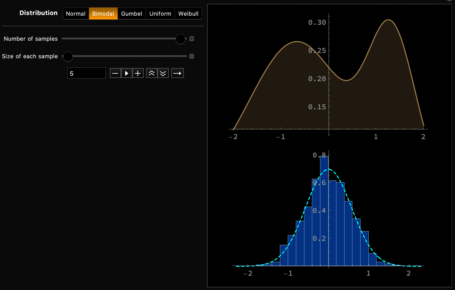
Demo
Central Limit Theorem
If \(X_1, X_2, \ldots, X_n\) are random samples from a population with mean \(\mu\) and finite standard deviation \(\sigma\), then the sum
\(\frac{X_1-\mu}{\sigma} + \frac{X_2-\mu}{\sigma} + \ldots + \frac{X_n-\mu}{\sigma}\)
will have a PDF that converges to \(\mathcal{N}(0, 1)\) in the limiting condition of \(n\to \infty\)

An alternative version of CLT
CLT - Attempt at Proof
If \(X_1, X_2, \ldots, X_n\) are random samples from a population with mean \(\mu\) and finite standard deviation \(\sigma\), then the sum
\(\frac{X_1-\mu}{\sigma} + \frac{X_2-\mu}{\sigma} + \ldots + \frac{X_n-\mu}{\sigma}\)
will have a PDF that converges to \(\mathcal{N}(0, 1)\) in the limiting condition of \(n\to \infty\)
What's strange about proving such a theorem?
We need to compare two PDFs !?


How do we test convergence as \(n\to\infty\) !?
CLT - Attempt at Proof
We need to compare two PDFs !?

Two PDFs can have the same \(\mu, \sigma\) and still differ
Exercise: Come up with an example
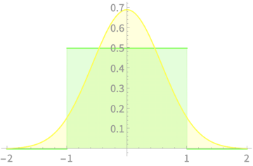
\(\mathcal{N}(0, 1/\sqrt{3})\)
\(\mathrm{Uniform}(-1, 1)\)
\(\mu = 0, \sigma = 1/\sqrt{3}\)
CLT - Attempt at Proof
We need to compare two PDFs !?

Two PDFs can have the same \(\mu, \sigma\) and still differ
\(\Rightarrow\) Need to compare more "terms"
These terms are called moments
\(\mathbb{E}[X^n]\)
\(= \sum_i x_i^n p(x_i)\), discrete
\( = \int_{-\infty}^\infty x^n f(x) dx\), continuous
The \(n\)th moment is given by
CLT - Attempt at Proof
We need to compare two PDFs !?

\(\mathbb{E}[X^n]\)
\(= \sum_i x_i^n p(x_i)\), discrete
\( = \int_{-\infty}^\infty x^n f(x) dx\), continuous
The \(n\)th moment is given by
Exercise: What is the 0th moment?
Answer: 1
CLT - Attempt at Proof
We need to compare two PDFs !?

\(\mathbb{E}[X^n]\)
\(= \sum_i x_i^n p(x_i)\), discrete
\( = \int_{-\infty}^\infty x^n f(x) dx\), continuous
The \(n\)th moment is given by
Exercise: What is the 1st moment?
Answer: \(\mu\)
CLT - Attempt at Proof
We need to compare two PDFs !?

\(\mathbb{E}[X^n]\)
\(= \sum_i x_i^n p(x_i)\), discrete
\( = \int_{-\infty}^\infty x^n f(x) dx\), continuous
The \(n\)th moment is given by
Exercise: What is the 2nd moment of the mean adjusted variable \(X = X' - \mu\)?
Answer: \(\sigma^2\)
CLT - Attempt at Proof
We need to compare two PDFs !?

\(\mathbb{E}[X^n]\)
\(= \sum_i x_i^n p(x_i)\), discrete
\( = \int_{-\infty}^\infty x^n f(x) dx\), continuous
The \(n\)th moment is given by
What is the 3rd moment of the mean, variance adjusted variable \(X = \frac{X' - \mu}{\sigma}\)?
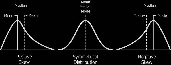
Answer: Turns out to be a measure of skewness
CLT - Attempt at Proof
We need to compare two PDFs !?

Thus to compare two PDFs we have to carefully match their moments

How do we test convergence as \(n\to\infty\) !?
What must be a property of a PDF that satisfies a convergence condition?

CLT - Attempt at Proof

How do we test convergence as \(n\to\infty\) !?
What must be a property of a PDF that satisfies a convergence condition?
Let \(Y_k = X_1 + X_2 + \ldots + X_k\), for all \(k\)
If \(Y_n \sim \mathcal{N}(\mu, \sigma)\),
then CLT requires that \(Y_{2n} \sim \mathcal{N}(\mu', \sigma')\)
The sum of two normally distributed r.v.s is also normally distributed?
CLT - Attempt at Proof

How do we test convergence as \(n\to\infty\) !?
The sum of two normally distributed r.v.s is also normally distributed?
Turns out to be true!
For two independent r.v.s
if \(X \sim \mathcal{N}(\mu_X, \sigma_X)\) and \(Y \sim \mathcal{N}(\mu_Y, \sigma_Y)\)
Then \(X+Y \sim \mathcal{N}(\mu_X + \mu_Y, \sqrt{\sigma_X^2 + \sigma_Y^2})\)
Exercise: Test this out graphically
CLT - Attempt at Proof

How do we test convergence as \(n\to\infty\) !?
Thus normal distribution is an attractor
Once the distribution becomes normal,
it remains normal
CLT - Attempt at Proof
If \(X_1, X_2, \ldots, X_n\) are random samples from a population with mean \(\mu\) and finite standard deviation \(\sigma\), then the sum
\(\frac{X_1-\mu}{\sigma} + \frac{X_2-\mu}{\sigma} + \ldots + \frac{X_n-\mu}{\sigma}\)
will have a PDF that converges to \(\mathcal{N}(0, 1)\) in the limiting condition of \(n\to \infty\)
What's strange about proving such a theorem?
We need to compare two PDFs !?


How do we test convergence as \(n\to\infty\) !?
Moments
Sum of normals
CLT - Implications
What use is CLT for data science?
Independent of PDF of population, PDF of \(\overline{X}\) is normal
Super elegant
" The mathematician does not study pure mathematics because it is useful; he studies it because he delights in it and he delights in it because it is beautiful.
- George Cantor
CLT - Implications
What use is CLT for data science?

PDF(\(X\))
PDF(\(\overline{X}\))
Independent of PDF of population, PDF of \(\overline{X}\) is normal
Super elegant
If we know (or guess) \(\mu, \sigma\) and have a measurement of \(\overline{X}\),
we can compute how likely is getting a value greater than \(\overline{X}\)
Likelihood of sample mean
CLT - Implications
What use is CLT for data science?
Exercise
Likelihood of sample mean
We have a population of die throws
We take a sample of 10 die throws
And find their total to be 40
How likely is it that we do better?
CLT - Implications
What use is CLT for data science?
Exercise
Likelihood of sample mean
We have a population of die throws
We take a sample of 10 die throws
And find their total to be 40
How likely is it that we do better?
Step 1
\(\mu = ?, \sigma = ?, n = ?\)
\(\mu = 3.5, \sigma = 1.708,\\ n = 10\)
Step 2
\(\mathbb{E}[X] = n\mu, \mathrm{sd}(X) =\sigma\sqrt{n}\)
\(\mathbb{E}[X] = 35, \mathrm{sd}(X) =5.401\)
Step 3
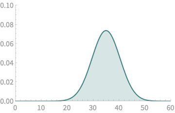
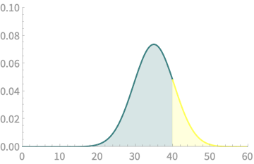
\(\mathcal{N}(35,5.41)\)
\(\mathrm{Pr}(X > 40) =\) Area of yellow part
CLT - Implications
What use is CLT for data science?
Likelihood of sample mean
Let us now see how we can compute such areas under \(\mathcal{N}\)
\(\mathrm{Pr}(X > 40) =\) Area of yellow part \(\approx 0.177\)
Given CLT, such area computations would always involve normal distributions

Computing area under \(\mathcal{N}\)
Key insight:
Relate \(\mathcal{N}(\mu, \sigma)\) for any \(\mu, \sigma\) to \(\mathcal{N}(0, 1)\)
Given \(X \sim \mathcal{N}(\mu, \sigma)\)
What can you say about \(Z = \frac{X - \mu}{\sigma}\)
We already have an intuition on this
Yes, \(Z \sim \mathcal{N}(0, 1)\)
This transformation of \(x \to \frac{x - \mu}{\sigma}\) is so important that we give it a name
Computing area under \(\mathcal{N}\)
This transformation of \(x \to \frac{x - \mu}{\sigma}\) is so important that we give it a name
Z Score
The number of standard deviations a value is away from the mean
\(z = \frac{x - \mu}{\sigma}\)
This is a generic definition for any random variable
Computing area under \(\mathcal{N}\)
Z Score
The number of standard deviations a value is away from the mean
\(z = \frac{x - \mu}{\sigma}\)
Examples
\(X \sim \mathcal{N}(0, 1)\)
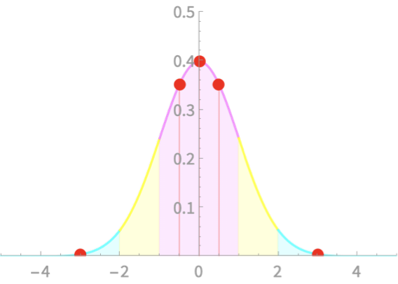
Calculate z-scores for x = -3, -0.5, 0, 0.5, 3
\(\mu = 0\). \(\sigma =1\)
| x | -3 | -0.5 | 0 | 0.5 | 3 |
| z |
Computing area under \(\mathcal{N}\)
Z Score
The number of standard deviations a value is away from the mean
\(z = \frac{x - \mu}{\sigma}\)
Examples
\(X \sim \mathcal{N}(0, 1)\)
Calculate z-scores for x = -3, -0.5, 0, 0.5, 3
\(\mu = 0\). \(\sigma =1\)
| x | -3 | -0.5 | 0 | 0.5 | 3 |
| z | -3 | -0.5 | 0 | 0.5 | 3 |
Computing area under \(\mathcal{N}\)
Z Score
The number of standard deviations a value is away from the mean
\(z = \frac{x - \mu}{\sigma}\)
Examples
\(X \sim \mathcal{N}(1, 2)\)
Calculate z-scores for x = -3, -0.5, 0, 0.5, 3
\(\mu = 1\). \(\sigma =2\)
| x | -3 | -0.5 | 0 | 0.5 | 3 |
| z |
Computing area under \(\mathcal{N}\)
Z Score
The number of standard deviations a value is away from the mean
\(z = \frac{x - \mu}{\sigma}\)
Examples
\(X \sim \mathcal{N}(1, 2)\)
Calculate z-scores for x = -3, -0.5, 0, 0.5, 3
\(\mu = 1\). \(\sigma =2\)
| x | -3 | -0.5 | 0 | 0.5 | 3 |
| z | -2 | -0.75 | -0.5 | -0.25 | 1 |
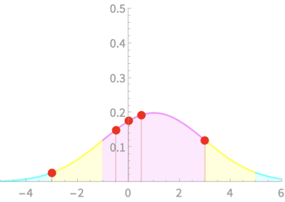
Computing area under \(\mathcal{N}\)
\(X \sim \mathcal{N}(1, 2)\)
\(\mu = 1\). \(\sigma =2\)
| x | -3 | -0.5 | 0 | 0.5 | 3 |
| z | -2 | -0.75 | -0.5 | -0.25 | 1 |
\(X \sim \mathcal{N}(0, 1)\)
\(\mu = 0\). \(\sigma =1\)
| x | -3 | -0.5 | 0 | 0.5 | 3 |
| z | -3 | -0.5 | 0 | 0.5 | 3 |

-ve Z score: Left of mean
+ve Z score: Right of mean
0 Z score: Exactly mean
Higher |Z score|: farther from mean, lower prob.

Computing area under \(\mathcal{N}\)
Z Score
The number of standard deviations a value is away from the mean
\(z = \frac{x - \mu}{\sigma}\)
Examples
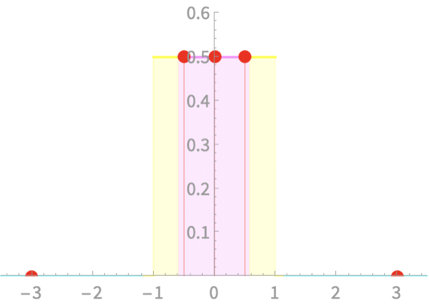
\(X \sim \mathrm{Uniform}[-1, 1]\)
Calculate z-scores for x = -2, -0.5, 0, 0.5, 2
\(\mu = 0\). \(\sigma =\frac{1}{\sqrt{3}} \approx 0.58\)
| x | -2 | -0.5 | 0 | 0.5 | 2 |
| z |
\(\mu = 0\). \(\sigma =?\)
\(\sigma^2 = \int_{-1}^1 (x - \mu)^2 f(x) dx\)
\(= \int_{-1}^1 (x - 0)^2 (1/2) dx\)
\(= \frac{1}{6} x^3|_{-1}^1\)
\(= \frac{1}{3}\)
Computing area under \(\mathcal{N}\)
Z Score
The number of standard deviations a value is away from the mean
\(z = \frac{x - \mu}{\sigma}\)
Examples
\(X \sim \mathrm{Uniform}[-1, 1]\)
Calculate z-scores for x = -2, -0.5, 0, 0.5, 2
\(\mu = 0\). \(\sigma =\frac{1}{\sqrt{3}} \approx 0.58\)
| x | -2 | -0.5 | 0 | 0.5 | 2 |
| z | -3.46 | -0.87 | 0 | 0.87 | 3.46 |
Computing area under \(\mathcal{N}\)
Z Score - Special Significance for \(\mathcal{N}\)
Given \(X \sim \mathcal{N}(\mu, \sigma)\) and \(Z = \frac{X - \mu}{\sigma}\)
Then, \(Z \sim \mathcal{N}(0, 1)\)
\(\mathrm{Pr}(X < a) \)
\(= \mathrm{Pr}\left(Z < \frac{a - \mu}{\sigma}\right)\)
\(= \mathrm{Pr}\left(\frac{X - \mu}{\sigma} < \frac{a - \mu}{\sigma}\right)\)
Seems simple, but effective!
Reduce all checks on to \(\mathcal{N}(0, 1)\)
Store in tables, and look-up!
Computing area under \(\mathcal{N}\)
Z Score - Special Significance for \(\mathcal{N}\)
Given \(X \sim \mathcal{N}(\mu, \sigma)\) and \(Z = \frac{X - \mu}{\sigma}\)
Then, \(Z \sim \mathcal{N}(0, 1)\)
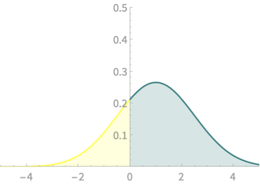
\(\mathrm{Pr}(X < a) \)
\(= \mathrm{Pr}\left(Z < \frac{a - \mu}{\sigma}\right)\)

Examples
\(X \sim \mathcal{N}(1, 1.5)\)
\(\mathrm{Pr}(X<0)\)
\(= \mathrm{Pr}(Z<\frac{0-1}{1.5})\)
Two yellow areas match
Computing area under \(\mathcal{N}\)
Z Score - Special Significance for \(\mathcal{N}\)
Given \(X \sim \mathcal{N}(\mu, \sigma)\) and \(Z = \frac{X - \mu}{\sigma}\)
Then, \(Z \sim \mathcal{N}(0, 1)\)
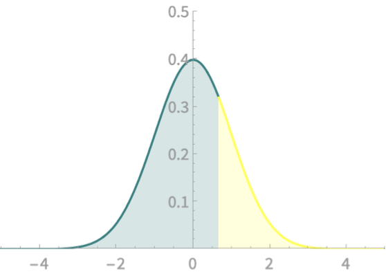
\(\mathrm{Pr}(X > a) \)
\(= \mathrm{Pr}\left(Z > \frac{a - \mu}{\sigma}\right)\)
Examples
\(X \sim \mathcal{N}(1, 1.5)\)
\(\mathrm{Pr}(X>2)\)
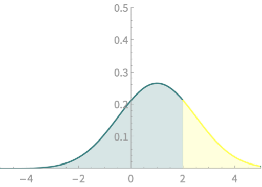
\(= \mathrm{Pr}(Z >\frac{2-1}{1.5})\)
Computing area under \(\mathcal{N}\)
Demo
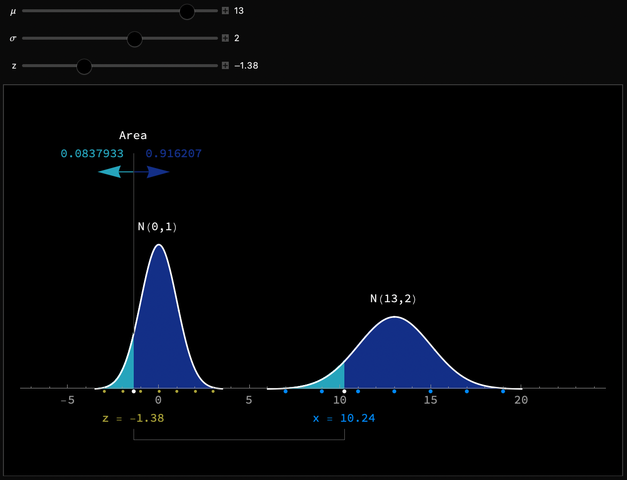
Computing area under \(\mathcal{N}\)
Efficiency in calculating
\(\mathrm{Pr}(X > a) \)
\(= \mathrm{Pr}\left(Z > \frac{a - \mu}{\sigma}\right)\)
When computers were expensive ...
Instead of computing \(\mathrm{Pr}(Z > c)\) each time, can we simply look-up in some tables?
Remember log tables from school?
Do we need to store \(\mathrm{Pr}(Z > c)\) for all values of \(c\). What about \(\mathrm{Pr}(Z < c)\)?
Computing area under \(\mathcal{N}\)
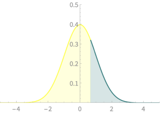
Some relations on the areas

+
= 1
\(\mathrm{Pr}(Z > a) + \mathrm{Pr}(Z \leq a) = 1\)
\(\mathrm{Pr}(Z > a) = \mathrm{Pr}(Z < -a) \)

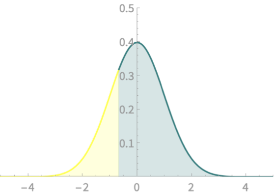
=
\(\mathrm{Pr}(Z < -3.5) \approx 0 \)
Computing area under \(\mathcal{N}\)
Some relations on the areas
\(\mathrm{Pr}(Z > a) + \mathrm{Pr}(Z \leq a) = 1\)
\(\mathrm{Pr}(Z > a) = \mathrm{Pr}(Z < -a) \)
\(\mathrm{Pr}(Z > 3.5) \approx 0 \)
Efficient table look-up
Sufficient to store \(\mathrm{Pr}(Z < a)\)
for \(a \in [-3.5, 0]\)
Computing area under \(\mathcal{N}\)
Efficient table look-up
Sufficient to store \(\mathrm{Pr}(Z < a)\)
for \(a \in [-3.5, 0]\)
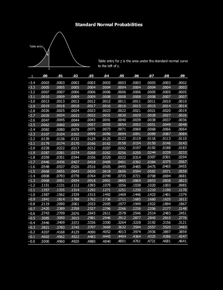

\(\mathrm{Pr}(Z < -2.81)\)
\(= .0025\)
Computing area under \(\mathcal{N}\)
Demo
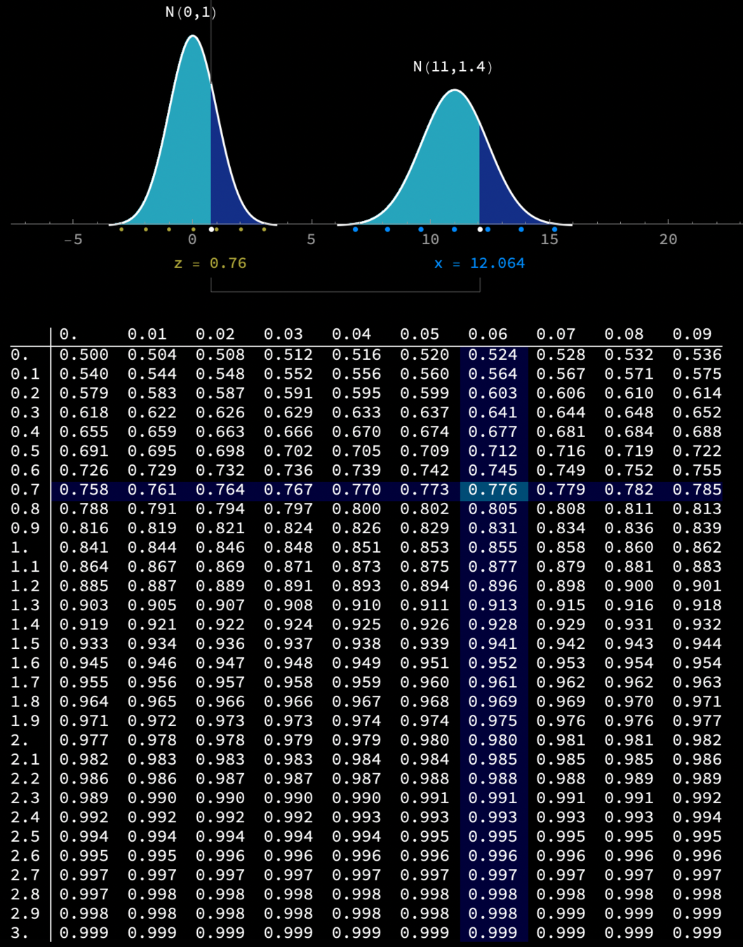
Computing area under \(\mathcal{N}\)
More areas
Given \(X \sim \mathcal{N}(\mu, \sigma)\) and \(Z = \frac{X - \mu}{\sigma}\)
Then, \(Z \sim \mathcal{N}(0, 1)\)
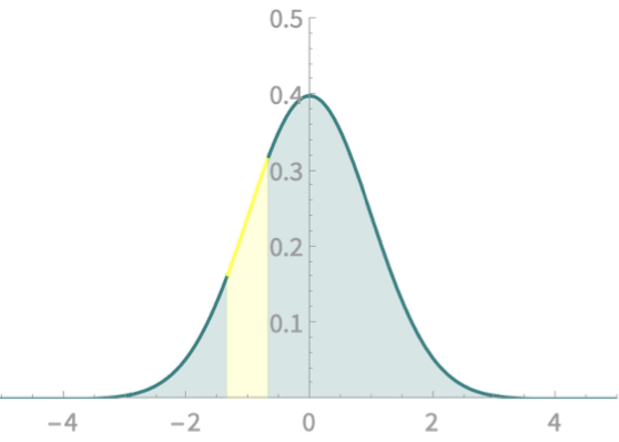
\(\mathrm{Pr}(a < X < b) \)
\(= \mathrm{Pr}\left(\frac{a - \mu}{\sigma} < Z < \frac{b - \mu}{\sigma}\right)\)
Examples
\(X \sim \mathcal{N}(1, 1.5)\)
\(\mathrm{Pr}(-1 < X<0)\)
\(= \mathrm{Pr}(\frac{-1-1}{1.5} < Z<\frac{0-1}{1.5})\)
Two yellow areas match
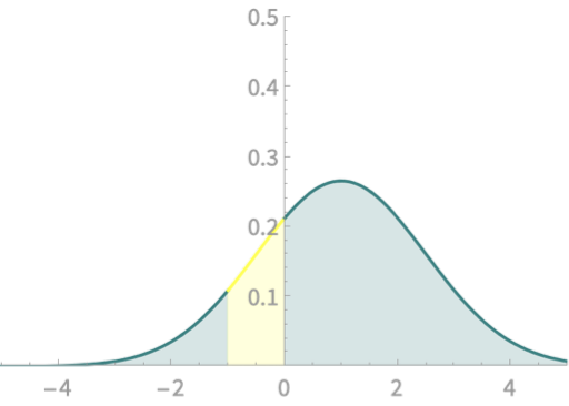
Computing area under \(\mathcal{N}\)
More areas
\(\mathrm{Pr}(\frac{-4}{3} < Z<\frac{-2}{3})\)

\(\mathrm{Pr}(Z<\frac{-2}{3})\)
\(\mathrm{Pr}( Z<\frac{-4}{3})\)
\(-\)
\(=\)

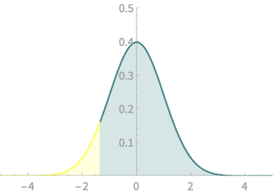
How will we compute this?
Two look-ups and subtraction
Back to our example
What use is CLT for data science?
Exercise
Likelihood of sample mean
We have a population of die throws
We take a sample of 10 die throws
And find their total to be 40
How likely is it that we do better?
Step 1
\(\mu = 3.5, \sigma = 1.708,\\ n = 10\)
Step 2
\(\mathbb{E}[X] = 35, \mathrm{sd}(X) =5.401\)
Step 3
\(\mathcal{N}(35,5.401)\)
\(\mathrm{Pr}(X > 40) =\) Area of yellow part

CLT - Implications
What use is CLT for data science?
Likelihood of sample mean
\(\mathcal{N}(35,5.401)\)
\(\mathrm{Pr}(X > 40) =\) Area of yellow part

\(= \mathrm{Pr}\left(Z > \frac{40 -35}{5.401}\right)\)
\(= \mathrm{Pr}\left(Z > 0.926\right)\)
\(= 0.177\)
We have a fighting chance to improve on 40!
CLT - Implications
What use is CLT for data science?
Likelihood of sample mean
\(\mathrm{Pr}(X > 40) \)
\(= 0.177\) (from CLT)
Let us check this without CLT
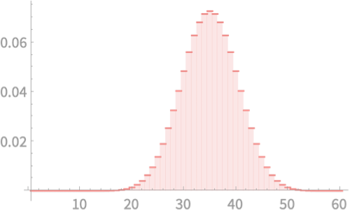
We can plot the PMF \(f(x)\) for each of the all possible values
\(\mathrm{Pr}(Q > 40) \)
\(= f(41) + f(42) + \ldots + f(60)\)
\(= 0.157\)
CLT - Implications
What use is CLT for data science?
Likelihood of sample mean
\(\mathrm{Pr}(X > 40) \)
\(= 0.177\) (from CLT)

\(\mathrm{Pr}(Q > 40) \)
\(= 0.157\) (PMF)
We have over-estimated our chance
Let us super-impose \(\mathcal{N}(35. 5.401)\)
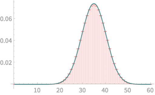
Looks good. Where did we go wrong!?
CLT - Implications
\(\mathrm{Pr}(X > 40) \)
\(= 0.177\) (from CLT)
\(\mathrm{Pr}(Q > 40) \)
\(= 0.157\) (PMF)

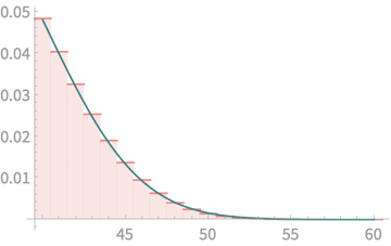
Let's zoom in
CLT - Implications
\(\mathrm{Pr}(X > 40) \)
\(= 0.177\) (from CLT)
\(\mathrm{Pr}(Q > 40) \)
\(= 0.157\) (PMF)

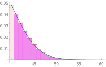
Let's zoom in
Map these values to areas


CLT - Implications
\(\mathrm{Pr}(X > 40) \)
\(= 0.177\) (from CLT)
\(\mathrm{Pr}(Q > 40) \)
\(= 0.157\) (PMF)

Let's zoom in


Yes we are overestimating
Alternative: Take yellow
area from 41
CLT - Implications
\(\mathrm{Pr}(X > 40) \)
\(= 0.177\) (from CLT)
\(\mathrm{Pr}(Q > 40) \)
\(= 0.157\) (PMF)


\(\mathrm{Pr}(X > 41) \)

\(= \mathrm{Pr}(Z > \frac{41-35}{5.401})\)
\(= 0.133\) (from CLT)
Ha! Underestimation
And its clear why
Why not 40.5?!
CLT - Implications
\(\mathrm{Pr}(X > 40) \)
\(= 0.177\) (from CLT)
\(\mathrm{Pr}(Q > 40) \)
\(= 0.157\) (PMF)

\(\mathrm{Pr}(X > 41) \)

\(= 0.133\) (from CLT)
\(\mathrm{Pr}(X > 40.5) \)
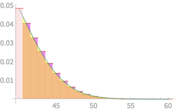
\(= \mathrm{Pr}(Z > 1.02 )\)
\(= 0.156\)
Neat!
CLT - Implications
\(\mathrm{Pr}(Q > 40) \)
\(= 0.157\) (PMF)

\(\mathrm{Pr}(X > 40.5) \)

\(= 0.156\) (CLT)
Continuity correction
CLT - Implications
\(\mathrm{Pr}(Q > 25 \) and \(Q < 36) \)

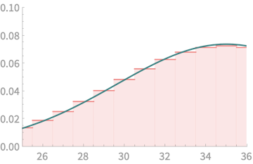
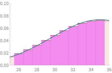
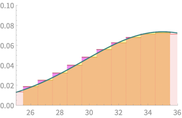
What we want to estimate
What we compute
\( = \mathrm{Pr}(X < 35.5) - \mathrm{Pr}( X < 25.5) \)
One more example
CLT - Implications
What use is CLT for data science?
Likelihood of sample mean
Approximating distributions
In a random group of 100 people, compute the PMF of number of people with birthdays on Tuesday
Recognise this distribution?
Binomial distribution
CLT - Implications
In a random group of 100 people, compute the PMF of number of people with birthdays on Tuesday
Binomial distribution
p = 1/7, n = 100
\(\mathrm{Pr}(Q = k) = \binom{n}{k} p^k (1-p)^{n - k}\)
Do this for 50 values of \(k\)
and you get a curve like this
\(\mathrm{Pr}(Q = k) \)
\(k\)
Expensive
to compute!

CLT - Implications
Binomial distribution
p = 1/7, n = 100
\(\mathrm{Pr}(Q = k) = \binom{n}{k} p^k (1-p)^{n - k}\)
\(\mathrm{Pr}(Q = k) \)
\(k\)
Let us plot \(\mathcal{N}(n\mu, \sqrt{n}\sigma) = \)
Pretty good approximation!
\(X\) can be seen as a the sum of 100 iid r.v.s with \(\mu = p = 1/7\) and \(\sigma = \sqrt{p(1-p)} \approx 0.35\)


\( \mathcal{N}(14.29, 0.35)\)
CLT - Implications
Using CLT
\(\mathrm{Pr}(Q = k) = \binom{n}{k} p^k (1-p)^{n - k}\)
\(k\)
Let \(X \sim \)

\( \mathcal{N}(14.29, 0.35)\)
\(\mathrm{Pr}(Q = k) \)
\(\approx\mathrm{Pr}(X < k + 0.5) - \mathrm{Pr}(X < k - 0.5)\)
\(k = 10\)
\(0.058\)
\(0.054\)
\(k = 15\)
\(0.109\)
\(0.111\)
\(k = 18\)
\(0.061\)
\(0.065\)
CLT - Implications
Normal approximation of binomial distribution
Demo
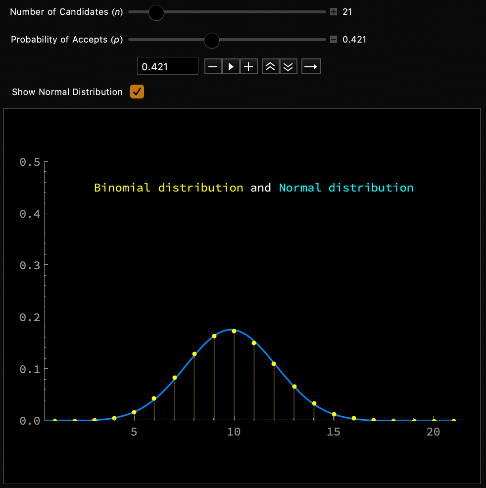
Insights
Higher accuracy for \(p \approx 0.5\)
Higher accuracy for larger \(n\)
Rule of thumb:
\(np > 10\) and \(n(1-p) > 10\)
CLT - Implications
What use is CLT for data science?
Likelihood of sample mean
Approximating distributions
Understanding bell curves in data
CLT - Implications
Understanding bell curves in data
A lot of real world data follows this trend
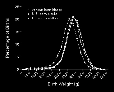
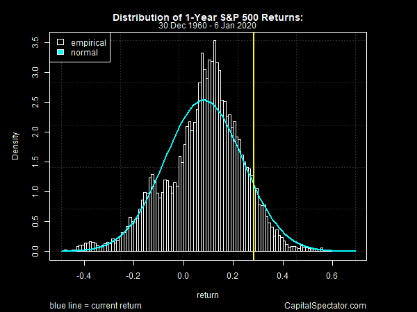
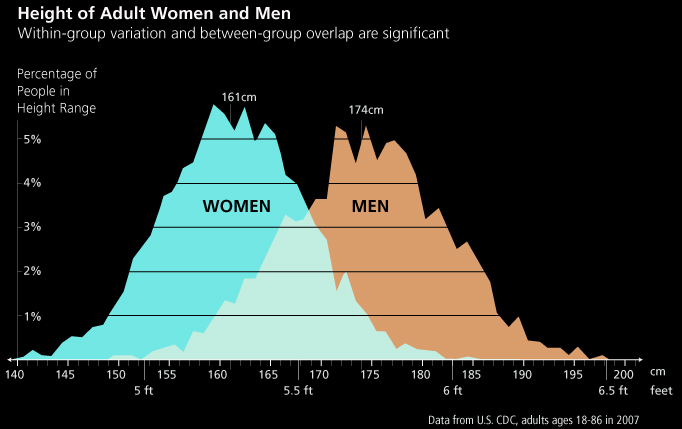
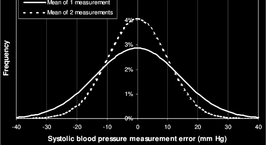
Weight of new-borns
Stock market returns
Measurement errors
Heights of adults
Not exactly \(\mathcal{N}\), but close
Why?
CLT - Implications
Understanding bell curves in data
If \(X_1, X_2, \ldots, X_n\) are random samples from a population with mean \(\mu\) and finite standard deviation \(\sigma\), then the sum
\(X_1 + X_2 + \ldots + X_n\)
will converge to \(\mathcal{N}(n\mu, \sigma\sqrt{n})\) in the limiting condition of \(n\to \infty\)
CLT so far
What happens if \(X_1, X_2, \ldots, X_n\) had different \(\mu, \sigma\)?
More general version of CLT
CLT - Implications
Understanding bell curves in data
More general version of CLT
If \(X_1, X_2, \ldots, X_n\) are independent random variables each with mean \(\mu_i\) and finite variance \(\sigma_i^2\), and let \(s^2_n = \sum_i^n \sigma_i^2\), then the sum
\(\sum_{i = 1}^{n}\frac{X_i - \mu_i}{s_n}\) converges in distribution to \(\mathcal{N}(0, 1)\) under some conditions*

* Roughly, no \(\sigma^2_i\) is comparable to the sum \(s_n^2\)
CLT - Implications
Understanding bell curves in data
General CLT
If \(X_1, X_2, \ldots, X_n\) are independent random variables each with mean \(\mu_i\) and finite variance \(\sigma_i^2\), and let \(s^2_n = \sum_i^n \sigma_i^2\), then the sum
\(\sum_{i = 1}^{n}\frac{X_i - \mu_i}{s_n}\) converges in distribution to \(\mathcal{N}(0, 1)\) under some conditions*
Implications?
If we can write a r.v. \(X\) as the sum of many many independent r.v.s,
Then \(X\) is likely to have a
bell-shaped distribution
CLT - Implications
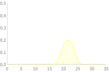
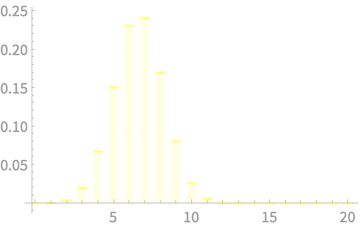
Example of sum of r.v.s
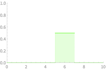
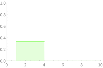
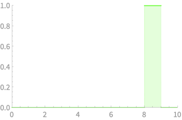
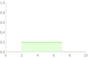
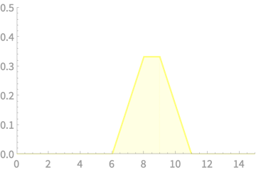
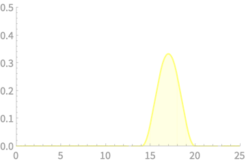
\(X_1\)
\(X_2\)
\(X_3\)
\(X_4\)
\(X_1 + X_2\)
\(X_1 + X_2 + X_3\)
\(X_1 + X_2 + X_3 + X_4\)
CLT - Implications
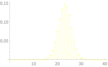
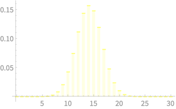
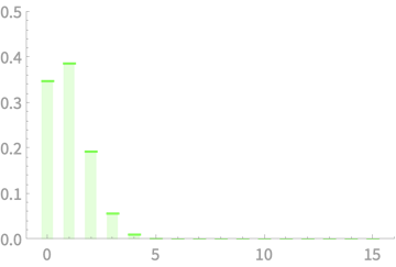
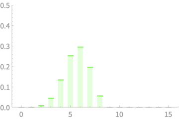
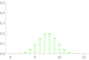
Example of sum of r.v.s
\(X_1\)
\(X_2\)
\(X_3\)
\(X_4\)
\(X_1 + X_2\)
\(X_1 + X_2 + X_3\)
\(X_1 + X_2 + X_3 + X_4\)
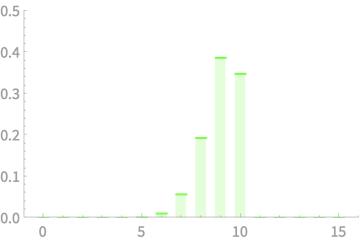
CLT - Implications
Understanding bell curves in data
Revisit examples


Weight of new-borns
Stock market returns
Measurement errors
Heights of adults
CLT - Implications
Choices we make
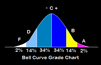
Grading in examinations
Check out how IQ scores are given
CLT - Implications
Choices we make
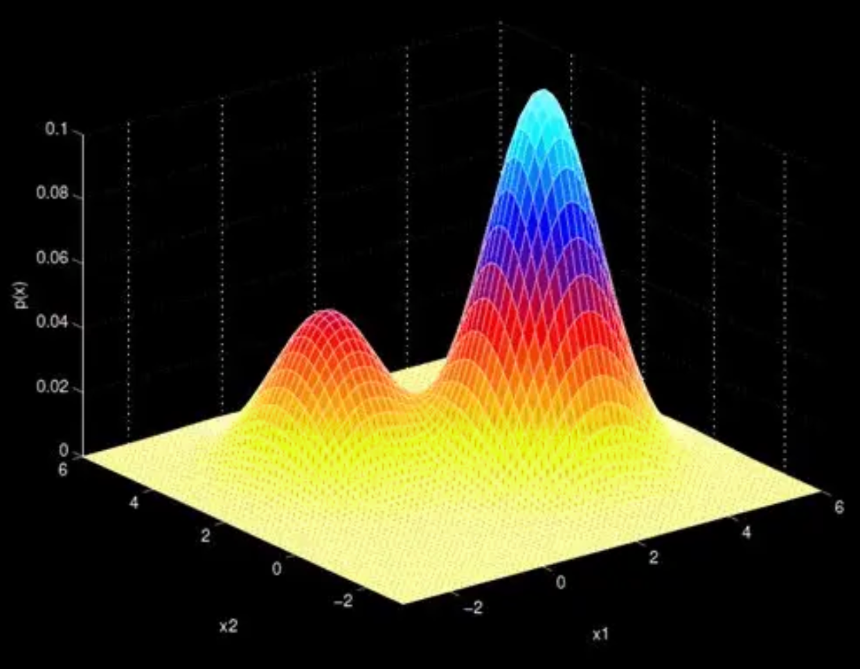
Fitting distributions in Machine Learning
Gaussian Mixture Models
Our Roadmap


Given \(\mu, \sigma\)
\(E(\bar{X})\), \(Var(\bar{X})\)
Central Limit Theorem
Given \(\mu, \sigma\)
\(E(S^2)\), \(Var(S^2)\)
Chi Square Distribution
Given \(p\)
\(E(\hat{p})\), \(Var(\hat{p})\)
Our Roadmap


Given \(\mu, \sigma\)
\(E(\bar{X})\), \(Var(\bar{X})\)
Central Limit Theorem
Given \(\mu, \sigma\)
\(E(S^2)\), \(Var(S^2)\)
Chi Square Distribution
Given \(p\)
\(E(\hat{p})\), \(Var(\hat{p})\)
Recap the big picture again
\(\Omega\)
Population size = \(N\)
Size of each sample = \(n\)
\(|\Omega| =\)\( N \choose n\)
\(F\)
0
1
\(P\)
\(\dfrac{1}{|\Omega|}\)


0
1
\(P\)
\(\dfrac{1}{|\Omega|}\)


\(X\)


10 km

40 km

5 km
\(S^2_{\tiny{mileage}}\)

\(Pr(S^2_{mileage})\)
Recap the big picture again
\(X = S^2\)


For each sample we want to compute the r.v. which is the sample variance
Then, we want to estimate \(\mathbb{E}[S^2]\) and \(\mathrm{var}(S^2)\) with \(\mu, \sigma\)
Computing \(S^2\)


What is the formula for \(S^2\)?
For a given sample,
\(S^2 = \frac{\sum_{i =1}^n (X_i - \overline{X})^2}{n}\)
Note that we compute the statistic with only information from the sample,
and not from the population

Estimating \(\mathbb{E}[S^2]\)
First Question
For a given sample, \(S^2 = \frac{\sum_{i =1}^n (X_i - \overline{X})^2}{n}\)
What is the relation of \(\mathbb{E}[S^2]\) to \(\mu, \sigma\)?
Exercise
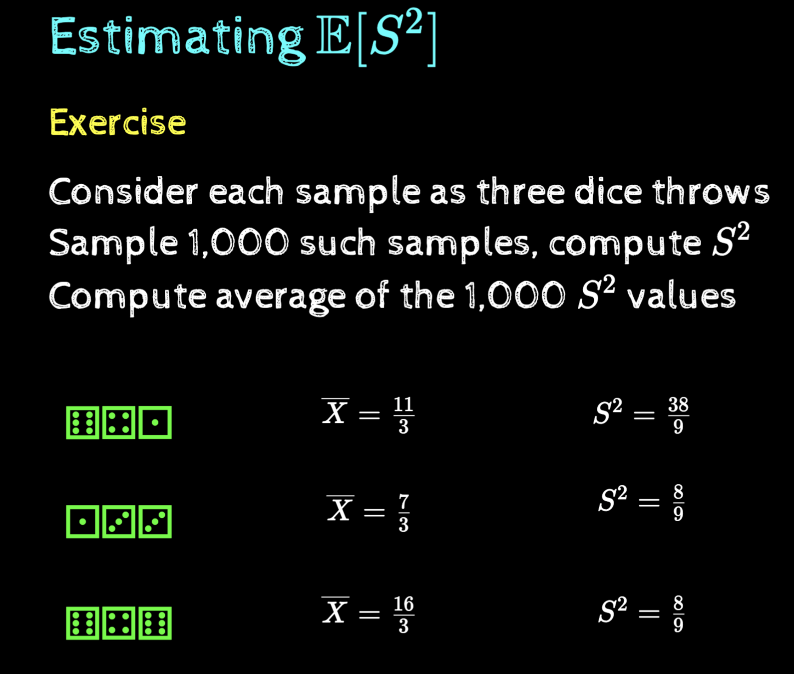
Consider each sample as three dice throws
Sample 1,000 such samples, compute \(S^2\)
Compute average of the 1,000 \(S^2\) values
What would you like it to be?
Estimating \(\mathbb{E}[S^2]\)
Exercise
Consider each sample as three dice throws
Sample 1,000 such samples, compute \(S^2\)
Compute average of the 1,000 \(S^2\) values
⚅⚃⚀
⚅⚃⚅
\(\overline{X} = \frac{11}{3}\)
⚀⚂⚂
\(\overline{X} = \frac{7}{3}\)
\(S^2 = \frac{8}{9}\)
\(S^2 = \frac{38}{9}\)
\(\overline{X} = \frac{16}{3}\)
\(S^2 = \frac{8}{9}\)
Estimating \(\mathbb{E}[S^2]\)
Exercise
Consider each sample as three dice throws
Sample 1,000 such samples, compute \(S^2\)
Compute average of the 1,000 \(S^2\) values
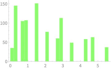
Average \(S^2 = 1.99\)
1000 samples
Estimating \(\mathbb{E}[S^2]\)
Exercise
Consider each sample as three dice throws
Sample 1,000 such samples, compute \(S^2\)
Compute average of the 1,000 \(S^2\) values
Average \(S^2 = 1.944\)
\(10^6\) samples
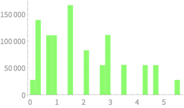
Estimating \(\mathbb{E}[S^2]\)
Exercise
Consider each sample as three dice throws
\(\mathbb{E}[S^2] \approx 1.944\)

\(\mu = 3.5, \sigma^2 = 2.916\)
We already know that for fair dice,
In this case, \(\mathbb{E}[S^2] < \sigma^2\)
Estimating \(\mathbb{E}[S^2]\)
Exercise
Let us take a continuous distribution
Sample 3 values from \(\mathcal{N}(0, 1)\)
Compute \(S^2\)
Repeat for 100,000 samples
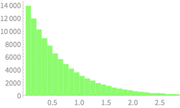
Average of \(S^2 = 0.665\)
Estimating \(\mathbb{E}[S^2]\)
Exercise
Sample 3 values from \(\mathcal{N}(0, 1)\)

Average of \(S^2 = 0.665\)
We know that \(\mu = 0, \sigma = 1\)
Again \(\mathbb{E}[S^2] < \sigma^2\)
We can play with two variables \(\mu\) and \(n\)
Estimating \(\mathbb{E}[S^2]\)
Exercise
Sample 3 values from \(\mathcal{N}(4, 1)\)

Average of \(S^2 = 0.666\) - Minor change
Again \(\mathbb{E}[S^2] < \sigma^2\)
Estimating \(\mathbb{E}[S^2]\)
Exercise
Sample 4 values from \(\mathcal{N}(0, 1)\)
Average of \(S^2 = 0.749\)
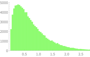
Again \(\mathbb{E}[S^2] < \sigma^2\)
Estimating \(\mathbb{E}[S^2]\)
Exercise
Sample 5 values from \(\mathcal{N}(0, 1)\)
Average of \(S^2 = 0.801\)
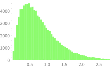
Plot the trend of \(\mathbb{E}[S^2]\) with \(n\)
Again \(\mathbb{E}[S^2] < \sigma^2\), but getting close
Estimating \(\mathbb{E}[S^2]\)
Exercise
Sample \(n\) values from \(\mathcal{N}(0, 1)\)
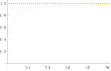
\(\mathbb{E}[S^2]\) & \(\sigma^2\) vs n
\(\mathbb{E}[S^2]\) \(\to\) \(\sigma^2\) as \(n \to \infty\)?
\(\mathbb{E}[S^2]\) is an under-estimate of \(\sigma^2\) and gets more accurate as sample size increases
Guess
Estimating \(\mathbb{E}[S^2]\)
\(S^2\) is an under-estimate of \(\sigma^2\) and gets more accurate as sample size increases
\(\mathbb{E}[S^2]\) \(= \mathbb{E}\left[\frac{\sum_{i = 1}^n(X_i - \overline{X})^2}{n}\right]\)
\(\mathbb{E}\left[\frac{\sum_{i = 1}^n(X_i - \mu)^2}{n}\right] = \) \(\sigma^2\)
We also know that \(\overline{X}\) is an unbiased estimate of \(\mu\)
Why then do we underestimate \(\sigma^2\) with \(\mathbb{E}[S^2]\)
We will see two arguments
Geometric and Algebraic
Estimating \(\mathbb{E}[S^2]\)
Why then do we underestimate \(\sigma^2\) with \(\mathbb{E}[S^2]\)
Geometric argument
\(\mathbb{E}\left[\frac{\sum_{i = 1}^n(X_i - \mu)^2}{n}\right] = \) \(\sigma^2\)
Consider the example of three dice throws
1
2
3
4
5
6
\(\mu = 3.5\)
⚀
Lets say we get 1, 3, 4
⚂
⚃
\(\overline{X} = 2.67\)
Average distance of samples from \(\overline{X}\)
\(\leq\) Average distance of samples from \(\mu\)
\(\mathbb{E}[S^2]\) \(= \mathbb{E}\left[\frac{\sum_{i = 1}^n(X_i - \overline{X})^2}{n}\right]\)
Estimating \(\mathbb{E}[S^2]\)
Why then do we underestimate \(\sigma^2\) with \(S^2\)
Geometric argument
\(\mathbb{E}\left[\frac{\sum_{i = 1}^n(X_i - \mu)^2}{n}\right] = \) \(\sigma^2\)
Consider the example of three dice throws
1
2
3
4
5
6
\(\mu = 3.5\)
⚀
Problem is less severe for spread out sample
⚂
⚅
\(\overline{X} = 3.33\)
There is still a small under-estimation
\(\mathbb{E}[S^2]\) \(= \mathbb{E}\left[\frac{\sum_{i = 1}^n(X_i - \overline{X})^2}{n}\right]\)
Estimating \(\mathbb{E}[S^2]\)
Why then do we underestimate \(\sigma^2\) with \(S^2\)
Geometric argument
\(\mathbb{E}\left[\frac{\sum_{i = 1}^n(X_i - \mu)^2}{n}\right] = \) \(\sigma^2\)
Consider the example of three dice throws
1
2
3
4
5
6
\(\mu = 3.5\)
⚀
Problem is severe for clustered samples
⚀
⚁
\(\overline{X} = 1.33\)
Such samples are rare, but not impossible
\(\mathbb{E}[S^2]\) \(= \mathbb{E}\left[\frac{\sum_{i = 1}^n(X_i - \overline{X})^2}{n}\right]\)
Estimating \(\mathbb{E}[S^2]\)
Why then do we underestimate \(\sigma^2\) with \(S^2\)
\(\mathbb{E}\left[\frac{\sum_{i = 1}^n(X_i - \mu)^2}{n}\right] = \) \(\sigma^2\)
In each case \(\mathbb{E}[S^2]\) \(<\) \(\sigma^2\)
1
2
3
4
5
6
⚀
⚀
⚁
1
2
3
4
5
6
⚀
⚂
⚅
1
2
3
4
5
6
⚀
⚂
⚃
\(\mathbb{E}[S^2]\) \(= \mathbb{E}\left[\frac{\sum_{i = 1}^n(X_i - \overline{X})^2}{n}\right]\)
Estimating \(\mathbb{E}[S^2]\)
Why then do we underestimate \(\sigma^2\) with \(S^2\)
\(\mathbb{E}\left[\frac{\sum_{i = 1}^n(X_i - \mu)^2}{n}\right] = \) \(\sigma^2\)
Algebraic argument
\( \sum_{i=1}^n(X_i - \mu)^2\)
\( =\sum_{i=1}^n((X_i - \overline{X})+(\overline{X} - \mu))^2\)
\( =\sum_{i=1}^n((X_i - \overline{X})^2+(\overline{X} - \mu)^2 + 2(X_i - \overline{X})(\overline{X} - \mu))\)
\(0\)
\( =\sum_{i=1}^n(X_i - \overline{X})^2+ \sum_{i =1}^n(\overline{X} - \mu)^2\)
Positive \(\Rightarrow\) underestimation
Relate this term to geometric argument
\(\mathbb{E}[S^2]\) \(= \mathbb{E}\left[\frac{\sum_{i = 1}^n(X_i - \overline{X})^2}{n}\right]\)
Estimating \(\mathbb{E}[S^2]\)
Let us find expected value of the error
\(\mathbb{E}[\sigma^2 - S^2]\)
\( = \mathbb{E}[\frac{1}{n}\sum_{i=1}^n (X_i - \mu)^2 - \frac{1}{n} \sum_{i = 1}^n(X_i - \overline{X})^2]\)
\( = \mathbb{E}[\frac{1}{n}\sum_{i=1}^n ((X_i^2 -2X_i\mu + \mu^2) - (X_i^2 - 2X_i\overline{X} + \overline{X}^2))]\)
\( = \mathbb{E}[\frac{1}{n}\sum_{i=1}^n (\mu^2 - \overline{X}^2 + 2X_i(\overline{X}-\mu)]\)
\( = \mathbb{E}[\mu^2 - \overline{X}^2 +\frac{1}{n} \sum_{i = 1}^n 2X_i(\overline{X}-\mu)]\)
\( = \mathbb{E}[\mu^2 - \overline{X}^2 +2\overline{X}(\overline{X}-\mu)]\)
\( = \mathbb{E}[\mu^2 + \overline{X}^2 -2\overline{X}\mu]\)
\( = \mathbb{E}[(\overline{X} - \mu)^2]\)
\( = \mathrm{Var}(\overline{X})\)
\( = \frac{\sigma^2}{n}\)
Estimating \(\mathbb{E}[S^2]\)
Let us find expected value of the error
\(\mathbb{E}[\sigma^2 - S^2]\)
\( = \frac{\sigma^2}{n}\)
\( = \frac{\sigma^2}{n}\)
\(\mathbb{E}[S^2] = \frac{n - 1}{n} \sigma^2\)

\(S^2\) & \(\sigma^2\) vs \(n\)
Now this plot
make senses
Estimating \(\mathbb{E}[S^2]\)
\(\mathbb{E}[S^2] = \frac{n - 1}{n} \sigma^2\)
We don't quite like this systematic error (bias)
We define an unbiased variance \(S_{n-1}^2\) as
\(\mathbb{E}[S^2_{n-1}] = \sigma^2\)
To distinguish, the usual biased variance is denoted \(S_n^2\) and given as
\(\mathbb{E}[S^2_{n}] = \frac{n - 1}{n}\sigma^2\)
Estimating \(\mathbb{E}[S^2]\)
\(\mathbb{E}[S^2_{n-1}] = \sigma^2\)
\(\mathbb{E}[S^2_{n}] = \frac{n - 1}{n}\sigma^2\)
In terms of sample data
\(S^2_{n}\) \(= \frac{\sum_{i = 1}^n (X_i - \overline{X})^2}{n}\)
\(S^2_{n-1}\) \(= \frac{\sum_{i = 1}^n (X_i - \overline{X})^2}{n-1}\)
Implications for Data Science
\(S^2_{n}\) \(= \frac{\sum_{i = 1}^n (X_i - \overline{X})^2}{n}\)
\(S^2_{n-1}\) \(= \frac{\sum_{i = 1}^n (X_i - \overline{X})^2}{n-1}\)
Sample mean \(\overline{X}\) is an unbiased estimate of \(\mu\)
With a small correction, the sample variance \(S^2_{n - 1}\) is an unbiased estimate of \(\sigma^2\)
Both of these hold independent of the distribution function
Implications for Data Science
\(S^2_{n}\) \(= \frac{\sum_{i = 1}^n (X_i - \overline{X})^2}{n}\)
\(S^2_{n-1}\) \(= \frac{\sum_{i = 1}^n (X_i - \overline{X})^2}{n-1}\)
Because there are two "values" of variance,
need to avoid confusion
In a numerical package, check which variance definition is used
The difference can be significant for small sample sizes
Our Roadmap


Given \(\mu, \sigma\)
\(E(\bar{X})\), \(Var(\bar{X})\)
Central Limit Theorem
Given \(\mu, \sigma\)
\(E(S^2)\), \(Var(S^2)\)
Chi Square Distribution
Given \(p\)
\(E(\hat{p})\), \(Var(\hat{p})\)
Our Roadmap


Given \(\mu, \sigma\)
\(E(\bar{X})\), \(Var(\bar{X})\)
Central Limit Theorem
Given \(\mu, \sigma\)
\(E(S^2)\), \(Var(S^2)\)
Chi Square Distribution
Given \(p\)
\(E(\hat{p})\), \(Var(\hat{p})\)
Estimating \(\mathrm{var}(S^2)\)
We will try to rewrite such that we have only one sampled value per term
\(S_{n-1}^2 = \frac{\sum_{i=1}^n (X_i - \overline{X})^2}{n-1}\)
In this term, there are two sampled quantities \(X_i\) and \(\overline{X}\) in each sum term
This is an example of such a term:
\(\sum_{i=1}^n\left(\frac{ X_i - \mu}{\sigma}\right)^2\)
Because we always want to work with independent random variables
Estimating \(\mathrm{var}(S^2)\)
\(\sum_{i=1}^n\left(\frac{ X_i - \mu}{\sigma}\right)^2\)
Let us play the algebraic tricks we have already seen
Estimating \(\mathrm{var}(S^2)\)
\(\sum_{i=1}^n\left(\frac{ X_i - \mu}{\sigma}\right)^2\)
\( = \sum_{i=1}^n\left(\frac{( X_i - \overline{X}) + (\overline{X} - \mu)}{\sigma}\right)^2\)
\( = \sum_{i = 1}^n\left(\frac{X_i - \overline{X}}{\sigma}\right)^2 + \sum_{i = 1}^n\left(\frac{\overline{X} - \mu}{\sigma}\right)^2 + 2 \left(\frac{\overline{X} - \mu}{\sigma^2}\right)\sum_{i = 1}^n(X_i - \overline{X})\)
\(0\)
\(S_{n-1}^2 = \frac{\sum_{i=1}^n (X_i - \overline{X})^2}{n-1}\)
\(\frac{(n-1)S_{n-1}^2}{\sigma^2} = \sum_{i=1}^n \left(\frac{X_i - \overline{X}}{\sigma}\right)^2\)
\( = \frac{(n-1)S^2_{n-1}}{\sigma^2} + \frac{n(\overline{X} - \mu)^2}{\sigma^2}\)
Estimating \(\mathrm{var}(S^2)\)
\(\sum_{i=1}^n\left(\frac{ X_i - \mu}{\sigma}\right)^2\)
\( = \frac{(n-1)S^2_{n-1}}{\sigma^2} + \frac{n(\overline{X} - \mu)^2}{\sigma^2}\)
Contains only a single random variable per term
What do these terms mean?
Turns out we cannot say much for any generic population distribution
Constrain \(X \sim \mathcal{N}(\mu, \sigma)\)
So what would we do?
Estimating \(\mathrm{var}(S^2)\)
\(\sum_{i=1}^n\left(\frac{ X_i - \mu}{\sigma}\right)^2\)
\( = \frac{(n-1)S^2_{n-1}}{\sigma^2} + \frac{n(\overline{X} - \mu)^2}{\sigma^2}\)
Constrain \(X \sim \mathcal{N}(\mu, \sigma)\)
Sum of squares of \(n\) i.i.d. r.v.s form a standard normal distribution
Square of one r.v. form a standard normal distribution
What do these terms mean?
What's the distribution of sum of squares of standard normal variables?
Our Roadmap


Given \(\mu, \sigma\)
\(E(\bar{X})\), \(Var(\bar{X})\)
Central Limit Theorem
Given \(\mu, \sigma\)
\(E(S)\), \(Var(S)\)
Chi Square Distribution
Given \(p\)
\(E(\hat{p})\), \(Var(\hat{p})\)
Our Roadmap


Given \(\mu, \sigma\)
\(E(\bar{X})\), \(Var(\bar{X})\)
Central Limit Theorem
Given \(\mu, \sigma\)
\(E(S)\), \(Var(S)\)
Chi Square Distribution
Given \(p\)
\(E(\hat{p})\), \(Var(\hat{p})\)
Chi Square Distribution
Let \(Z_1, Z_2, \ldots, Z_n\) be independent standard normal variables and \(Q = \sum_{i = 1}^n Z_i^2\)
Then, what is the distribution of \(Q\)?
Let us try plotting
for \(n = 1, 2, 3, \ldots\)
Chi Square Distribution
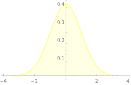
\(Z_1\)
What will happen if we square it?
\(Q = Z_1^2\)
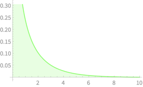
\(Q\)
Chi Square Distribution

\(Z_1\)
\(Q = Z_1^2 + Z_2^2\)

\(Z_2\)
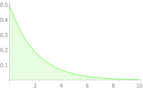
\(Q\)
Chi Square Distribution

\(Z_1\)
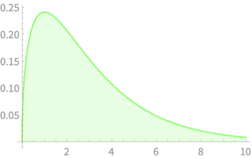
\(Q = Z_1^2 + Z_2^2 + Z_3^2\)

\(Z_2\)

\(Z_3\)
\(Q\)
Chi Square Distribution

\(Z_1\)
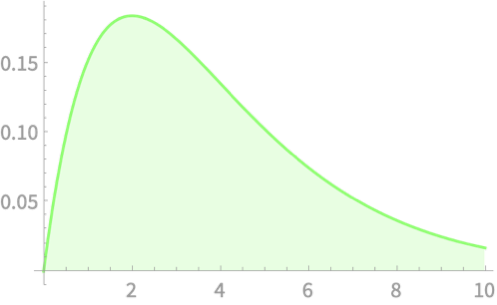
\(Q = Z_1^2 + Z_2^2 + Z_3^2 + Z_4^2\)

\(Z_2\)

\(Z_3\)

\(Z_4\)
\(Q\)
Chi Square Distribution

\(Z_1\)
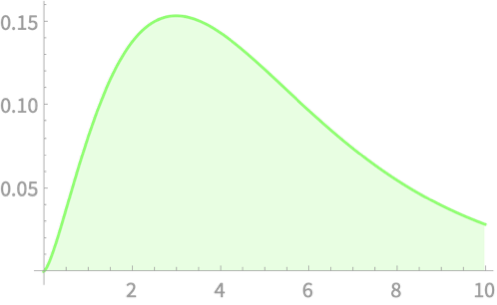
\(Q = Z_1^2 + Z_2^2 + Z_3^2 + Z_4^2 + Z_5^2\)

\(Z_2\)

\(Z_3\)

\(Z_4\)

\(Z_5\)
\(Q\)
Chi Square Distribution
\(Q = Z_1^2 + Z_2^2 + Z_3^2 + \ldots + Z_{100}^2\)
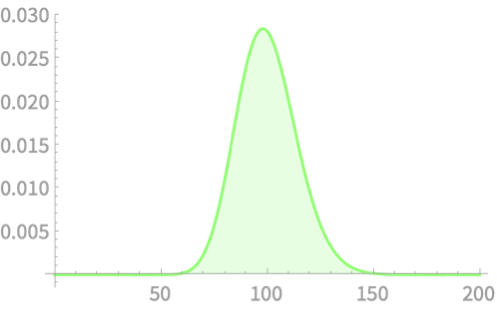
We cannot escape the normal curve can we?!
Chi Square Distribution
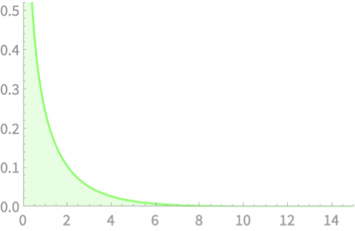
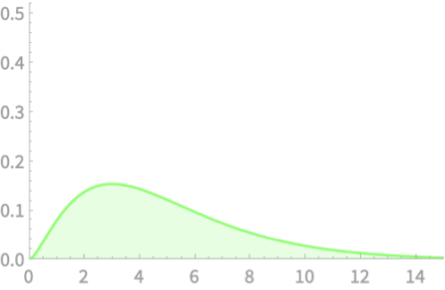
\(Q = Z_1^2\)
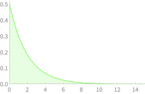
\(Q = Z_1^2 + Z_2^2\)
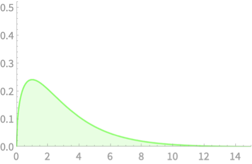
\(Q = Z_1^2 + Z_2^2 + Z_3^2\)
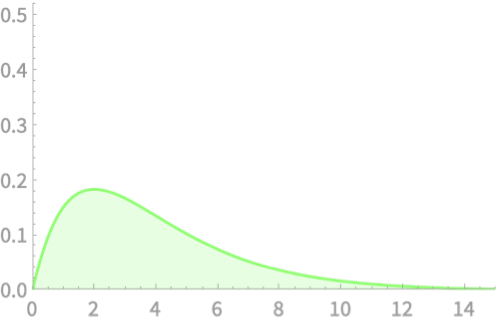
\(Q = Z_1^2 + Z_2^2 + Z_3^2 + Z_4^2\)
\(Q = Z_1^2 + Z_2^2 + Z_3^2 + Z_4^2 + Z_5^2\)
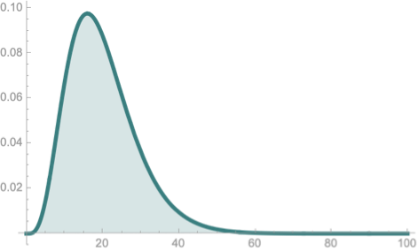
\(Q \sim \chi^2(1)\)
\(Q \sim \chi^2(2)\)
\(Q \sim \chi^2(3)\)
\(Q \sim \chi^2(4)\)
\(Q \sim \chi^2(5)\)
Chi Square Distribution
\(\chi^2(k)\) has \(k\) degrees of freedom
Chi Square Distribution

\(Q = Z_1^2 + Z_2^2 + Z_3^2 + Z_4^2\)
\(Q \sim \chi^2(4)\)
Chi-square distribution with \(k\) degrees of freedom \(\chi^2(k)\)
If \(Q\) is the sum of squares of \(k\) independent standard normal variables then \(Q \sim \chi^2(k)\)
Natural follow-up questions:
What are the mean and variance of \(\chi^2(k)\)
Chi Square Distribution
Mean of \(\chi^2(k)\)
Let us start with \(\chi^2(1)\)
\(\mu_{\chi^2(1)} = \mathbb{E}[Z^2]\), where \(Z\sim \mathcal{N}(0, 1)\)
Where have we seen \(\mathbb{E}[Z^2]\)?
\(\sigma^2(Z) = \mathbb{E}[Z^2] - (\mathbb{E}[Z])^2\)
\(1= \mathbb{E}[Z^2] - 0\)
\(\mathbb{E}[Z^2] = 1\)
\(\Rightarrow \mathbb{E}[Q] = 1\)

\(Q = Z_1^2\)
\(Q \sim \chi^2(1)\)

\(Z_1\)
Relate to the plots
Chi Square Distribution
Mean of \(\chi^2(k)\)
\(\mathbb{E}[Z^2] = 1\)

\(Q = Z_1^2 + Z_2^2\)
\(Q \sim \chi^2(2)\)
On to mean of \(\chi^2(2)\)
\(\mathbb{E}[Q] = \mathbb{E}[Z_1^2 + Z_2^2]\)
\(=\mathbb{E}[Z_1^2] + \mathbb{E}[Z_2^2]\)
Since \(Z_1\) and \(Z_2\) are independent
\(=2\)
Chi Square Distribution
Mean of \(\chi^2(k)\)
\(\mathbb{E}[Z^2] = 1\)

\(Q = Z_1^2 + Z_2^2\)
\(Q \sim \chi^2(2)\)
On to mean of \(\chi^2(2)\)
\(\mathbb{E}[Q] = \mathbb{E}[Z_1^2 + Z_2^2]\)
\(=\mathbb{E}[Z_1^2] + \mathbb{E}[Z_2^2]\)
\(=2\)

\(Q = Z_1^2\)
\(Q \sim \chi^2(1)\)
Mean shifts to the right with an added degree of freedom
Chi Square Distribution


Extending this argument, we have the nice result that
Mean of \(\chi^2(k) = k\)
Chi Square Distribution
Variance of \(\chi^2(k)\)
\(\sigma^2(Z^2) = \mathbb{E}[Z^4] - (\mathbb{E}[Z^2])^2\)
Let us start with \(\mathrm{var}(\chi^2(1))\)
\(\mathbb{E}[Z^4]\) recall is a moment of the normal distribution - the 4th moment or Kurtosis
We can compute it with the integral
\(\int_{-\infty}^\infty x^4 f(x) dx\), where \(f(x)\) is the PDF of \(\mathcal{N}(0, 1)\)
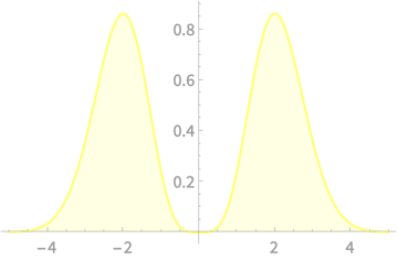
\(\int_{-\infty}^\infty x^4 f(x) dx\)
Area under this curve is 3
\(= 3 - 1 = 2\)
Chi Square Distribution
Variance of \(\chi^2(k)\)
\(\mathrm{var}(\chi^2(1)) = 2\)
Consider \(Q = Z_1^2 + Z_2^2\)
\(\mathrm{var}(Q) = \mathrm{var}(Z_1^2 + Z_2^2)\)
\(= \mathrm{var}(Z_1^2) + \mathrm{var}(Z_2^2)\)
Since \(Z_1\) and \(Z_2\) are independent
\(= 2 + 2 = 4\)
\(\mathrm{var}(\chi^2(k)) = 2k\)
Chi Square Distribution
\(\chi^2(k)\) is the distribution of the sum of the squares of \(k\) standard normal distributions
\(k\) is referred to as the degrees of freedom
Mean of \(\chi^2(k)\) is \(k\) and variance is \(2k\)

Chi Square Distribution
Implications in data science
Being a close relative to \(\mathcal{N}\), you will find that \(\chi^2\) is a commonly used distribution
Applications (some in this course)
Quantify goodness of fit
Test independence of two variables
Confidence interval estimation for \(\sigma^2\)
Our Roadmap


Given \(\mu, \sigma\)
\(E(\bar{X})\), \(Var(\bar{X})\)
Central Limit Theorem
Given \(\mu, \sigma\)
\(E(S^2)\), \(Var(S^2)\)
Chi Square Distribution
Given \(p\)
\(E(\hat{p})\), \(Var(\hat{p})\)
Our Roadmap


Given \(\mu, \sigma\)
\(E(\bar{X})\), \(Var(\bar{X})\)
Central Limit Theorem
Given \(\mu, \sigma\)
\(E(S^2)\), \(Var(S^2)\)
Chi Square Distribution
Given \(p\)
\(E(\hat{p})\), \(Var(\hat{p})\)
Recap: Estimating \(\mathrm{var}(S^2)\)
\(\sum_{i=1}^n\left(\frac{ X_i - \mu}{\sigma}\right)^2\)
\( = \frac{(n-1)S^2_{n-1}}{\sigma^2} + \frac{n(\overline{X} - \mu)^2}{\sigma^2}\)
What's the distribution of sum of squares of standard normal variables?
Constrain \(X \sim \mathcal{N}(\mu, \sigma)\)
Sum of squares of \(n\) i.i.d. r.v.s form a standard normal distribution
Square of one r.v. form a standard normal distribution
What do these terms mean?
\(\chi^2\) distributions
Estimating \(\mathrm{var}(S^2)\)
\(\sum_{i=1}^n\left(\frac{ X_i - \mu}{\sigma}\right)^2\)
\( = \frac{(n-1)S^2_{n-1}}{\sigma^2} + \frac{n(\overline{X} - \mu)^2}{\sigma^2}\)
Sum of squares of \(n\) i.i.d. r.v.s form a standard normal distribution
Square of one r.v. form a standard normal distribution
\(\sim \chi^2(n)\)
\(\sim \chi^2(1)\)
Estimating \(\mathrm{var}(S^2)\)
\(\sum_{i=1}^n\left(\frac{ X_i - \mu}{\sigma}\right)^2\)
\( = \frac{(n-1)S^2_{n-1}}{\sigma^2} + \frac{n(\overline{X} - \mu)^2}{\sigma^2}\)
\(\sim \chi^2(n)\)
\(\sim \chi^2(1)\)
By equating the moments of LHS and RHS and using some uniqueness theorems
\(\sim \chi^2(n-1)\)
\(\frac{(n-1)S^2_{n - 1}}{\sigma^2}\) has a \(\chi^2\) distribution with
\(n - 1\) degrees of freedom
Estimating \(\mathrm{var}(S^2)\)
\(\sum_{i=1}^n\left(\frac{ X_i - \mu}{\sigma}\right)^2\)
\( = \frac{(n-1)S^2_{n-1}}{\sigma^2} + \frac{n(\overline{X} - \mu)^2}{\sigma^2}\)
\(\frac{(n-1)S^2_{n - 1}}{\sigma^2}\) has a \(\chi^2\) distribution with
\(n - 1\) degrees of freedom
\(S_{n-1}^2 = \frac{\sum_{i=1}^n (X_i - \overline{X})^2}{n-1}\)
If we freely choose \(n-1\) terms, the last one gets fixed
What's with the
degree of freedom?!
\(\sum_{i=1}^n (X_i - \overline{X}) = 0\)
\(S^2_{n-1}\) has \(n\) terms adding up, but they are not independent
Because of this we lose one degree of freedom
Estimating \(\mathrm{var}(S^2)\)
\(\frac{(n-1)S^2_{n - 1}}{\sigma^2}\) has a \(\chi^2\) distribution with
\(n - 1\) degrees of freedom
Now that we have the distribution, lets check the mean value
We already knew \(\mathbb{E}[S^2_{n - 1}] = \sigma^2\)
\(\mathbb{E}\left[\frac{(n-1)S^2_{n-1}}{\sigma^2}\right]= \) Mean of \(\chi^2(n - 1)\)
\(\Rightarrow \frac{(n-1)}{\sigma^2}\mathbb{E}\left[S^2_{n-1}\right]= n - 1\)
\(\Rightarrow \mathbb{E}\left[S^2_{n-1}\right]= \sigma^2\)
Estimating \(\mathrm{var}(S^2)\)
\(\frac{(n-1)S^2_{n - 1}}{\sigma^2}\) has a \(\chi^2\) distribution with
\(n - 1\) degrees of freedom
Now that we have the distribution, lets estimate the variance
\(\mathrm{var}\left(\frac{(n-1)S^2_{n-1}}{\sigma^2}\right)= \) \(\mathrm{var}\) of \(\chi^2(n - 1)\)
\(\Rightarrow \frac{(n-1)^2}{\sigma^4}\mathrm{var}(S^2_{n-1})= \) \(2(n - 1)\)
\(\mathrm{var}(aX) = a^2\mathrm{var}(X)\)
\(\Rightarrow \mathrm{var}(S^2_{n-1})= \) \(\frac{2\sigma^4}{n - 1}\)
Satistics of \(S^2\)
The sample statistic \(S^2_{n-1}\) defined as \(\frac{\sum_{i = 1}^n (X - \overline{X})^2}{n-1}\) is an unbiased estimator of the population variance \(\sigma^2\), i.e., \(\mathbb{E}(S^2_{n -1}) = \sigma^2\)

If the population values are normally distributed, then \(\frac{(n - 1)S^2_{n - 1}}{\sigma^2} \sim \chi^2(n - 1)\) and \(\mathrm{var}(S^2_{n - 1}) = \frac{2\sigma^4}{n - 1}\)

On to Experiments
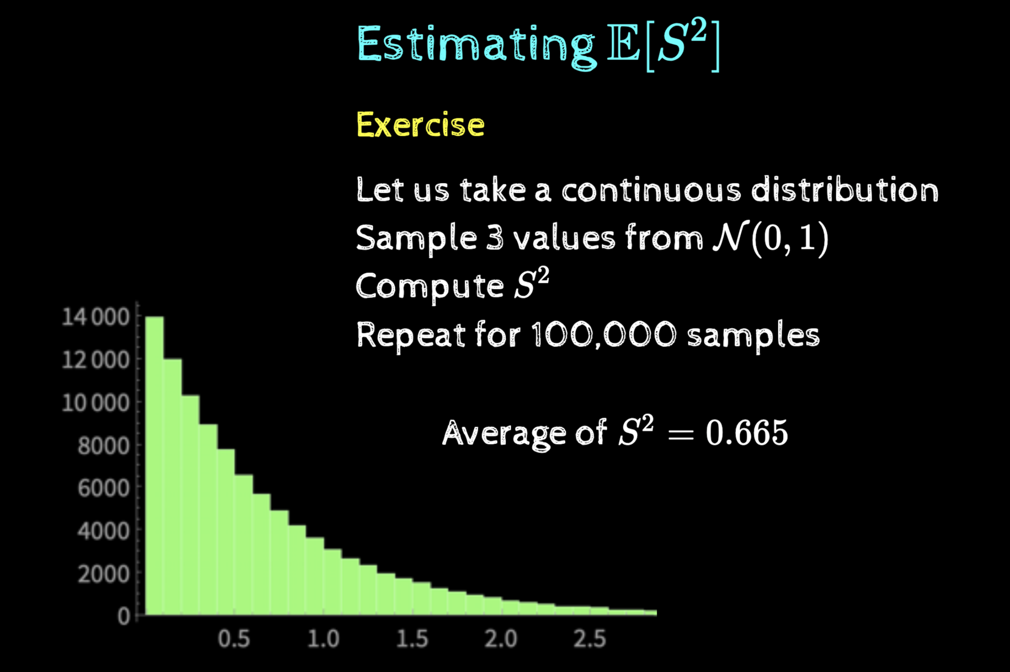
Recall our earlier examples
On to Experiments
Recall our earlier examples
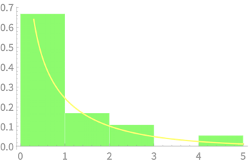
Distribution of variance of 2 values sampled from \(\mathcal{N}(0, 1)\)
Now we know that we should use unbiased variance \(S^2_{n - 1}\)
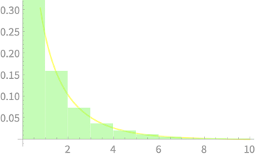
Measured distribution of \((n - 1)S^2_{n - 1}\)
vs \(\chi^2(1)\)
Histogram vs PDF
count is normalized
bin width = 1
On to Experiments
Recall our earlier examples
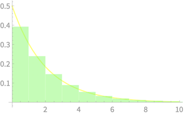
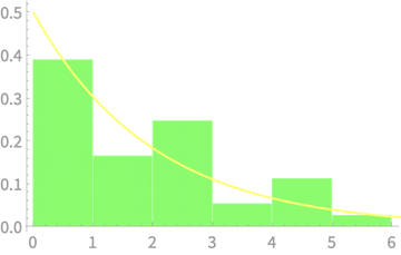
Distribution of variance of 3 values sampled from \(\mathcal{N}(0, 1)\)
Measured distribution of \((n - 1)S^2_{n - 1}\)
vs \(\chi^2(2)\)
On to Experiments
Recall our earlier examples
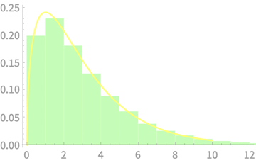
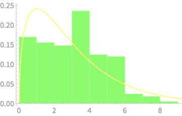
Distribution of variance of 4 values sampled from \(\mathcal{N}(0, 1)\)
Measured distribution of \((n - 1)S^2_{n - 1}\)
vs \(\chi^2(3)\)
On to Experiments
Recall our earlier examples
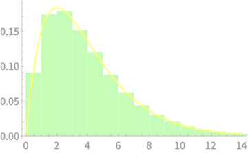
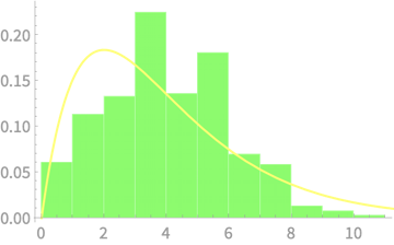
Distribution of variance of 5 values sampled from \(\mathcal{N}(0, 1)\)
Measured distribution of \((n - 1)S^2_{n - 1}\)
vs \(\chi^2(4)\)
On to Experiments
Our other example on dice
The underlying distribution is not normal and thus we cannot estimate the distribution
On to Experiments
Sample of \(n\) dice throws
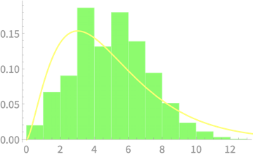
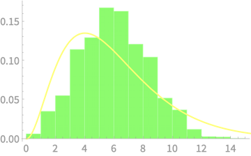
\(n = 2\)
\(n = 3\)
\(n = 4\)
\(n = 5\)
\(n = 7\)
\(n = 8\)
Measured
\((n - 1)S^2_{n - 1}\)
vs \(\chi^2(4)\)
Our Roadmap


Given \(\mu, \sigma\)
\(E(\bar{X})\), \(Var(\bar{X})\)
Central Limit Theorem
Given \(\mu, \sigma\)
\(E(S)\), \(Var(S)\)
Chi Square Distribution
Given \(p\)
\(E(\hat{p})\), \(Var(\hat{p})\)
Our Roadmap


Given \(\mu, \sigma\)
\(E(\bar{X})\), \(Var(\bar{X})\)
Central Limit Theorem
Given \(\mu, \sigma\)
\(E(S^2)\), \(Var(S^2)\)
Chi Square Distribution
Given \(p\)
\(E(\hat{p})\), \(Var(\hat{p})\)
Recall Example
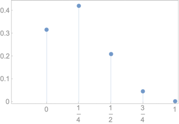
Proportion as a statistic measure of fraction of card sets that contain King of Diamonds
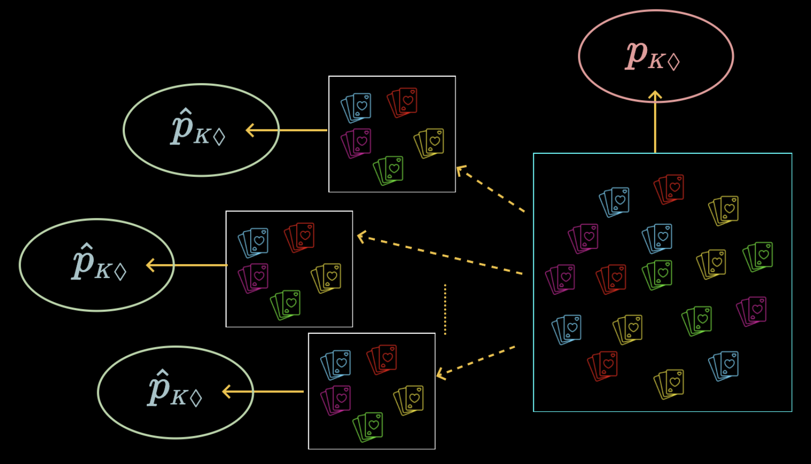
Expectation of Proportion
Let us formalise this new statistic

\(p\) - Proportion of elements in population satisfying a condition
\(\hat{p}\) - Proportion of elements in sample satisfying a condition
We already know about \(\mathbb{E}[\overline{X}]\) and \(\mathbb{E}[S]\)
Can we somehow relate \(\mathbb{E}[\hat{p}]\) to these?
Expectation of Proportion
Exercise

Define a random variable such that its sample mean is related to \(\hat{p}\)
Indicator variable
Define a random variable \(X\) such that
\(= 0\), otherwise
\(X_i = 1\), if \(i\)th element of sample satisfies condition
Expectation of Proportion

Indicator variable
Define a random variable \(X\) such that
\(= 0\), otherwise
\(X_i = 1\), if \(i\)th element of sample satisfies condition
How is \(\hat{p}\) related to \(X\)?
Expectation of Proportion

Indicator variable
Define a random variable \(X\) such that
\(= 0\), otherwise
\(X_i = 1\), if \(i\)th element of sample satisfies condition
How is \(\hat{p}\) related to \(X\)?
\(\hat{p} = \frac{X_1 + X_2 + \ldots X_n }{n}\)
\(= \overline{X}\)
Expectation of Proportion
Indicator variable
\(= 0\), otherwise
\(X_i = 1\), if \(i\)th element of sample satisfies condition
\(\hat{p} = \overline{X}\)
For \(X\), what is the population mean \(\mu\)?

We are asking for the mean of the indicator variable for all elements in the population
\(\mu = \frac{\sum_{i = 1}^N X_i}{N} \)
\(=p \)
Expectation of Proportion
Indicator variable
\(= 0\), otherwise
\(X_i = 1\), if \(i\)th element of sample satisfies condition
\(\hat{p} = \overline{X}\)

\(\mu = p\)
We already know that \(\mathbb{E}[\overline{X}]= \mu\)
\(\Rightarrow \mathbb{E}[\hat{p}] = \mathbb{E}[\overline{X}] = \mu = p\)
Expectation of Proportion

\(\mathbb{E}[\hat{p}] = p\)
Sample statistics of proportion are unbiased estimates of the population parameter of proportion
Variance of Proportion

Indicator variable
\(= 0\), otherwise
\(X_i = 1\), if \(i\)th element of sample satisfies condition
\(\mathbb{E}[\overline{X}] = p\)
What is \(\mathrm{var}(\overline{X})\) ?
Variance of Proportion

Indicator variable
\(= 0\), otherwise
\(X_i = 1\), if \(i\)th element of sample satisfies condition
\(\mathbb{E}[\overline{X}] = p\)
For the indicator variable \(X\) what is the corresponding population parameter \(\sigma\)?
True
False
PMF
\(p\)
\(1 - p\)
\(\sigma^2 = \frac{\sum_{i = 1}^N (X - \mu)^2}{N}\)
\(= p(1-p)^2 + (1-p)(0 - p)^2\)
\(= p(1-p)\)
Variance of Proportion

Indicator variable
\(= 0\), otherwise
\(X_i = 1\), if \(i\)th element of sample satisfies condition
\(\mathbb{E}[\overline{X}] = p\)
For the indicator variable \(X\) what is the corresponding population parameter \(\sigma\)?
True
False
PMF
\(p\)
\(1 - p\)
\(\sigma\)
\(= \sqrt{p(1-p)}\)
Variance of Proportion

Indicator variable
\(= 0\), otherwise
\(X_i = 1\), if \(i\)th element of sample satisfies condition
\(\mathbb{E}[\overline{X}] = p\)
\(\sigma\)
\(= \sqrt{p(1-p)}\)
What is \(\mathrm{var}(\overline{X})\)?
\(\mathrm{var}(\overline{X}) = \frac{\sigma^2}{n}\)
\(= \frac{p(1-p)}{n}\)
\(= \mathrm{var}(\hat{p})\)
Variance of Proportion
\(\mathbb{E}[\hat{p}] = p\)
\(\mathrm{var}(\hat{p}) \)
\(= \frac{p(1-p)}{n}\)
What is the maximum value of \(\mathrm{var}(\hat{p})\) for a given \(n\)?
True
False
PMF
\(p = 0.25 \Rightarrow \mathrm{var}(\hat{p}) = \frac{0.1875}{n}\)
Variance of Proportion
\(\mathbb{E}[\hat{p}] = p\)
\(\mathrm{var}(\hat{p}) \)
\(= \frac{p(1-p)}{n}\)
What is the maximum value of \(\mathrm{var}(\hat{p})\) for a given \(n\)?
True
False
PMF
\(p = 0.5 \Rightarrow \mathrm{var}(\hat{p}) = \frac{0.25}{n}\)
Variance of Proportion
\(\mathbb{E}[\hat{p}] = p\)
\(\mathrm{var}(\hat{p}) \)
\(= \frac{p(1-p)}{n}\)
What is the maximum value of \(\mathrm{var}(\hat{p})\) for a given \(n\)?
True
False
PMF
\(p = 0.75 \Rightarrow \mathrm{var}(\hat{p}) = \frac{0.1875}{n}\)
\(\mathrm{var}(\hat{p})\) is highest when \(p = 0.5\)
Variance of Proportion
\(\mathbb{E}[\hat{p}] = p\)
\(\mathrm{var}(\hat{p}) \)
\(= \frac{p(1-p)}{n}\)
Let us take up our original problem

Recall that an outcome is a random set of 13 cards from a standard deck
\(\mathbb{E}[\hat{p}] = p = \frac{1}{4}\)
If our samples consist of \(n = 5\) such sets of 13 cards, what are statistics of \(\hat{p}\)
\(p = 1/4\)
\(\mathrm{var}(\hat{p}) = \frac{p(1 - p)}{n} = \frac{3}{80}\)
Variance of Proportion
\(\mathbb{E}[\hat{p}] = p\)
\(\mathrm{var}(\hat{p}) \)
\(= \frac{p(1-p)}{n}\)
Let us take up our original problem

Recall that an outcome is a random set of 13 cards from a standard deck
\(\mathbb{E}[\hat{p}] = p = \frac{1}{4}\)
If our samples consist of \(n = 20\) such sets of 13 cards, what are statistics of \(\hat{p}\)
\(p = 1/4\)
\(\mathrm{var}(\hat{p}) = \frac{p(1 - p)}{n} = \frac{3}{320}\)
Satistics of \(\hat{p}\)
\(= 0\), otherwise
\(X_i = 1\), if \(i\)th element of sample satisfies condition
The sample statistic \(\hat{p}\) as defined as the proportion of the population satisfying a boolean condition is related to the indicator random variable

\(\mathbb{E}[\hat{p}] = p\)
\(\mathrm{var}(\hat{p}) \)
\(= \frac{p(1-p)}{n}\)
The statistics of \(\hat{p}\) are given as
Our Roadmap
