Recap: List of Topics
Descriptive Statistics
Probability Theory
Inferential Statistics
Different types of data
Different types of plots
Measures of centrality and spread
Sample spaces, events, axioms
Discrete and continuous RVs
Bernoulli, Uniform, Normal dist.
Sampling strategies
Interval Estimators
Hypothesis testing (z-test, t-test)
ANOVA, Chi-square test
Linear Regression
What is the effect of transformations on percentiles?
Learning Objectives
What are percentiles?
What are the different measures of spread?
How do you compute the percentile rank of a value in the data?
What are box plots and how to use them to visualise some measures of centrality and spread?
What is the effect of transformations on measures of spread?
What are some frequently used percentiles?
What are percentiles?
Intuition: Percentiles
Suppose you scored 45 out of 100 on a test, how would you rate your performance? Good or bad?

Example
Is it bad? (because you scored less than 50%)

But ... ...
What if the questions were really hard?

What if the time provided was insufficient?

Intuition: Percentiles
Suppose you scored 45 out of 100 on a test. Out of 100 students, only 2 scored greater than 45. How do you rate your performance?

Example
Does it look good now?

Yes, it does ... ...

You can proudly say that you lie in the top 98 percentile of your class (the score of 98% of students was less than or equal to your score)
Percentiles
A university conducts a written test for 25 students and decides to call those students for an interview whose score is above the 70th percentile

Example
44, 43, 37, 68, 55, 46, 19, 59, 34, 46, 51, 62, 47, 52, 44, 28, 36, 56, 65, 60, 55, 66, 54, 48, 62
Can you Identify which students will be called for the interview?

Percentiles
25 students (sorted scores)
The p percentile of a sample is a value such that p perentage of the values in the data are less than or equal to this value

70-th percentile
sorted data values
19, 28, 34, 36, 37, 43, 44, 44, 46, 46, 47, 48, 51, 52, 54, 55, 55, 56, 59, 60, 62, 62, 65, 66, 68
Percentiles
25 students (sorted scores)
Sort the data
Compute location of the p-th percentile

The 70th percentile lies at location 18.2 !
19, 28, 34, 36, 37, 43, 44, 44, 46, 46, 47, 48, 51, 52, 54, 55, 55, 56, 59, 60, 62, 62, 65, 66, 68
Percentiles
25 students (sorted scores)
Where is the position 18.2?
56
59
19, 28, 34, 36, 37, 43, 44, 44, 46, 46, 47, 48, 51, 52, 54, 55, 55
60, 62, 62, 65, 66, 68

18.2 is between 18 and 19, closer to 18

The 70th percentile should be between 56 and 59, greater than 56 but closer to 56
Percentiles

What is the overall procedure?
Sort the data
Compute location of the p-th percentile
integer part of
fractional part of
18
0.2
Compute p-th percentile as
Percentiles (some more intuition)

if is high then the weightage given to will be lower than that given to and vice versa
Percentiles
19, 28, 34, 36, 37, 43, 44, 44, 46, 46, 47, 48, 51, 52, 54, 55, 55, 56, 59, 60, 62, 62, 65, 66, 68
Percentiles
A university conducts a written test for 25 students and decides to call those students for an interview whose score is above the 70th percentile

Example
The school will invite only those 7 students whose score was greater than 56.6
19, 28, 34, 36, 37, 43, 44, 44, 46, 46, 47, 48, 51, 52, 54, 55, 55, 56, 59, 60, 62, 62, 65, 66, 68

Percentiles
Suppose the school changes its decision and now only wants to invite students who scored greater than 80 percentile

Example
60
62
19, 28, 34, 36, 37, 43, 44, 44, 46, 46, 47, 48, 51, 52, 54, 55, 55, 56, 59
62, 65, 66, 68
Percentiles
Suppose the school changes its decision and now only wants to invite students who scored greater than 80 percentile

Example
60
62
19, 28, 34, 36, 37, 43, 44, 44, 46, 46, 47, 48, 51, 52, 54, 55, 55, 56, 59
62, 65, 66, 68
Percentiles
60
62
19, 28, 34, 36, 37, 43, 44, 44, 46, 46, 47, 48, 51, 52, 54, 55, 55, 56, 59
62, 65, 66, 68

Why did we have to compute ? Wasn't knowing enough to identify the shortlisted students?
Yes, it was, but the university may also be required to declare the cut-off score, hence we need to compute. also
Suppose there were only 24 students and p=80

Example
Percentiles (special case: )
60
19, 28, 34, 36, 37, 43, 44, 44, 46, 46, 47, 48, 51, 52, 54, 55, 55, 56, 59
62, 62, 65, 66

In such cases the percentile would actually correspond to a value in the data
What are some alternative methods found in textbooks?
Alternative 1
Sort the data
Compute location of the p-th percentile
integer part of
Alternative 2
Marks of 24 students and interested in p=70

Example
(note the use of n instead of n+1)
Alternative 2
Sort the data
Compute location of the p-th percentile
integer part of
(note the use of n instead of n+1)
Alternative 2
Marks of 25 students and p=70 or p=80

Example
19, 28, 34, 36, 37, 43, 44, 44, 46, 46, 47, 48, 51, 52, 54, 55, 55, 56, 59, 60, 62, 62, 65, 66, 68
Alternative 2: intuition
the p-th percentile is that value in the data such that at least p percentage of the values are less than or equal to it and at least (100-p) percentage of the values are greater than it

At least 17.5 values should be less than or equal to it (so the location should be 18 or higher)
At least 7.5 values should be greater than or equal to it (so the location should be 18 or lower)
Location 18 (i.e., ) is the only location which satisfies both conditions
19, 28, 34, 36, 37, 43, 44, 44, 46, 46, 47, 48, 51, 52, 54, 55, 55, 56, 59, 60, 62, 62, 65, 66, 68
Alternative 2: intuition
the p-th percentile is that value in the data such that at least p percentage of the values are less than or equal to it and at least (100-p) percentage of the values are greater than it

Both locations 20 and 21 (i.e., ) satisfy the above conditions so just take an average of these two values
19, 28, 34, 36, 37, 43, 44, 44, 46, 46, 47, 48, 51, 52, 54, 55, 55, 56, 59, 60, 62, 62, 65, 66, 68
Alternative 3
Sort the data
Compute location of the p-th percentile
integer part of
(same as alternative 1)
(same as alternative 1)
(same as alternative 1 except that use 0.5 instead of )
Comparison
19, 28, 34, 36, 37, 43, 44, 44, 46, 46, 47, 48, 51, 52, 54, 55, 55, 56, 59, 60, 62, 62, 65, 66, 68
Alternative 1
Alternative 2
Case 1
is integer
Case 2
is not integer
Alternative 3
P = 70
P = 80
What are some frequently used percentiles?
Quartiles
19, 28, 34, 36, 37
Quartiles divide the data into four equal parts

43, 44, 44, 46, 46
47, 48, 51, 52, 54
55, 55, 56, 59, 60
Quartiles: Example
Shikhar Dhawan T20I scores (50 sorted scores)
0, 1, 1, 1, 1, 1, 2, 2, 3, 3, 4, 5, 5, 5, 5, 6, 6, 8, 9, 10, 10, 11, 13, 14, 15, 16, 23, 23, 24, 26, 29, 30, 30, 32, 33, 35, 41, 42, 43, 46, 47, 51, 55, 60, 72, 74, 76, 80, 90, 92
Median is same as Q2
median

Are they the same?
(of course, the are !)

But why do the formulae look different?
Median is same as Q2
Case 1: n is odd
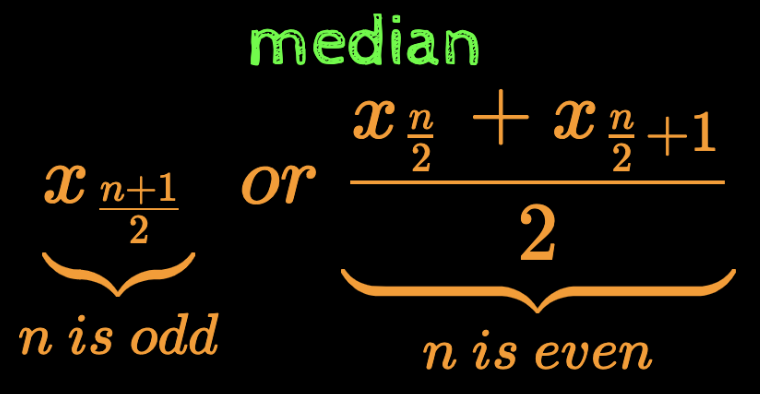
Case 1: n is even
Median is same as Q2
Quintiles
19, 28, 34, 36
Quintiles divide the data into five equal parts

37, 43, 44, 44
46, 46, 47, 48
55, 56, 59, 60
51, 52, 54, 55
Quintiles: Example
Shikhar Dhawan T20I scores (50 sorted scores)
0, 1, 1, 1, 1, 1, 2, 2, 3, 3, 4, 5, 5, 5, 5, 6, 6, 8, 9, 10, 10, 11, 13, 14, 15, 16, 23, 23, 24, 26, 29, 30, 30, 32, 33, 35, 41, 42, 43, 46, 47, 51, 55, 60, 72, 74, 76, 80, 90, 92
Similarly you can compute the other 8 deciles!
Deciles
Deciles divide the data into five equal parts

19,28 34,36 37,43 44,44 46,46 47,48 51,52 54,55 55,56 59,60
Deciles: Example
Shikhar Dhawan T20I scores (50 sorted scores)
0, 1, 1, 1, 1, 1, 2, 2, 3, 3, 4, 5, 5, 5, 5, 6, 6, 8, 9, 10, 10, 11, 13, 14, 15, 16, 23, 23, 24, 26, 29, 30, 30, 32, 33, 35, 41, 42, 43, 46, 47, 51, 55, 60, 72, 74, 76, 80, 90, 92
Similarly you can compute the other 8 deciles!
How to compute the percentile rank of a value in the data?
44, 43, 37, 68, 55, 46, 19, 59, 34, 46, 51, 62, 47, 52, 44, 28, 36, 56, 65, 60, 55, 66, 54, 48, 62
Percentile Rank

Compared to other students, how do you rate the performance of the student who scored 44?

What is the percentile rank of the student who scored 44
OR
The percentile rank of a value is the percentage of data values that are less than on equal to it

Percentile Rank: Example 1
19, 28, 34, 36, 37, 43, 44, 44, 46, 46, 47, 48, 51, 52, 54, 55, 55, 56, 59, 60, 62, 62, 65, 66, 68
Percentile Rank: Example 2
Shikhar Dhawan T20I scores (59 sorted scores)
0, 1, 1, 1, 1, 1, 2, 2, 3, 3, 3, 4, 5, 5, 5, 5, 6, 6, 8, 9, 10, 10, 11, 13, 14, 15, 16, 19, 23, 23, 23, 24, 26, 29, 30, 30, 31, 32, 32, 33, 35, 36, 40, 41, 41, 42, 43, 46, 47, 51, 52, 55, 60, 72, 74, 76, 80, 90, 92
We typically round it upto the next whole number (65 in this case)
What is the effect of transformations on percentiles?
Transformations
Scaling and Shifting
(a = 5/9, c = -160/9)
Temperature in Fahrenheit:
[22.46, 23.54, 24.26, 27.86, 30.2, 30.74, 34.52, 35.96, 40.46, 44.06, 52.7, 54.68, 56.66, 57.56, 59.54, 61.52, 62.06, 65.66, 67.46, 70.88, 76.46, 82.4, 83.12, 84.38, 93.02, 94.28, 95.72, 96.44, 108.86, 109.58]
Temperature in Celsius:
[-5.3, -4.7, -4.3, -2.3, -1.0, -0.7, 1.4, 2.2, 4.7, 6.7, 11.5, 12.6, 13.7, 14.2, 15.3, 16.4, 16.7, 18.7, 19.7, 21.6, 24.7, 28.0, 28.4, 29.1, 33.9, 34.6, 35.4, 35.8, 42.7, 43.1]
bad aesthetics
Effect of transformations (on percentiles)
Effect of transformations (on percentiles)
Temperature in Fahrenheit:
[22.46, 23.54, 24.26, 27.86, 30.2, 30.74, 34.52, 35.96, 40.46, 44.06, 52.7, 54.68, 56.66, 57.56, 59.54, 61.52, 62.06, 65.66, 67.46, 70.88, 76.46, 82.4, 83.12, 84.38, 93.02, 94.28, 95.72, 96.44, 108.86, 109.58]
Temperature in Celsius:
[-5.3, -4.7, -4.3, -2.3, -1.0, -0.7, 1.4, 2.2, 4.7, 6.7, 11.5, 12.6, 13.7, 14.2, 15.3, 16.4, 16.7, 18.7, 19.7, 21.6, 24.7, 28.0, 28.4, 29.1, 33.9, 34.6, 35.4, 35.8, 42.7, 43.1]
bad aesthetics
Summary
p-th percentile
sorted data values
Percentile (definition)
How to compute percentiles?
(alternative methods not recommended)
Summary
Frequently used percentiles
How to compute percentile rank of a value?
Quartiles
Quintiles
Deciles
What is the effect of transformations on percentiles?
What are the measures of spread?
Motivation: Measures of spread
Sample 1: 81, 81, 82, 82, 83, 83, 84, 84, 85, 85 Mean: 83
Median: 83
Sample 1: 31, 41, 61, 72, 83, 83, 94, 105, 125, 135 Mean: 83
Median: 83
All values are very close to the mean & median (low variability in data)
Some values are far from the mean & median (high variability in data)

Measures of centrality don't tell us anything about the spread and variability in the data
Measures of spread (range)
Sample 1: 81, 81, 82, 82, 83, 83, 84, 84, 85, 85 Mean: 83
Median: 83
Sample 1: 31, 41, 61, 72, 83, 83, 94, 105, 125, 135 Mean: 83
Median: 83

Range clearly tells us that the second sample has more variability/spread than the first
Range: (max value - min value) = 85 - 81 = 4
Range: (max value - min value) = 135 - 31 = 104
Measures of spread (range)
Farm yields of wheat (in bushels): 40.1, 40.9, 41.8, 44, 46.8, 47.2, 48.6, 49.3, 49.4, 51.9, 53.8, 55.9, 57.3, 58.1, 60.2, 60.7, 61.1, 61.4, 62.8, 633
Just like the mean, the range is very sensitive to outliers!
data of some 20 farms in one state or district such that one farm has a very high production and hence is an outlier (at least 10 times the production of the second maximum in the data)
Range: (max value - min value) = 633 - 40.1 = 592.9
Note that most values were close to 40.1 : the range however is blown up due to one outlier (633)

40.1, 40.9, 41.8, 44, 46.8
47.2, 48.6, 49.3, 49.4, 51.9
53.8, 55.9, 57.3, 58.1, 60.2
60.7, 61.1, 61.4, 62.8, 633
replace the data in the table with the same data as on the previous slide
Measures of spread (IQR)
replace the data in the table with the same data as on the previous slide
fill in the values of xx, yy and zz
Measures of spread (IQR)
40.1, 40.9, 41.8, 44, 46.8
47.2, 48.6, 49.3, 49.4, 51.9
53.8, 55.9, 57.3, 58.1, 60.2
60.7, 61.1, 61.4, 62.8, 633
40.1, 40.9, 41.8, 44, 46.8
47.2, 48.6, 49.3, 49.4, 51.9
53.8, 55.9, 57.3, 58.1, 60.2
60.7, 61.1, 61.4, 62.8, 633
replace the data in the table with the same data as on the previous slide
fill in the values of xx, yy and zz
put a cross on the outlier
fragments: table, IQR, cross, L_75, highlight 15th element in the data, L_25, highlight 5th element in the data, IQr^new
Measures of spread (IQR)

Clearly not sensitive to outliers (i.e,, will not change if we drop the outlier)

40.1, 40.9, 41.8, 44, 46.8
47.2, 48.6, 49.3, 49.4, 51.9
53.8, 55.9, 57.3, 58.1, 60.2
60.7, 61.1, 61.4, 62.8, 633
Measures of spread (variance)
Question: How different are the values in the data from the typical value (mean) in the data?
Possible Solution: Compute the sum or average deviation of all points from the mean
Issue: We already know that the sum of deviations from the mean is 0
Motivation: Measures of spread
Sample 1: 81, 81, 82, 82, 83, 83, 84, 84, 85, 85 Mean: 83
Median: 83
Sample 1: 31, 41, 61, 72, 83, 83, 94, 105, 125, 135 Mean: 83
Median: 83
Sum of deviations = 0

The sum of deviations does not tell us anything about the spread of the data
Sum of deviations = 0
Measures of spread (variance)
Observation: We do not care about the sign of the deviation (Both positive and negative deviations contribute to the spread in the data and hence we do want them to cancel each other)
Deviations on left side
Deviations on right side
Mean: 6.0
1 2 3 4 5 6 7 8 9 10
=
Measures of spread (variance)
Issue: The sum of deviations from the mean is 0
Reason: The positive deviations cancel the negative deviations
Solution1: Use absolute values
Solution1: Use square values
preferred solution
Measures of spread (variance)
Variance:
(if computed from a sample)
(if computed from the entire population)
Why is there a difference in the formula?

We will clarify this later once we introduce probability theory
Measures of spread (variance)
show two tables: one corresponding to each of the samples on slide 55
the tables will have the following columns: x, x-x_bar, (x-x_bar)^2
the columns will appear one by one
81
81
82
82
83
83
84
84
85
85
2
2
1
1
0
0
1
1
2
2
4
4
1
1
0
0
1
1
4
4
31
41
61
72
83
83
94
105
125
135
2
2
1
1
0
0
1
1
2
2
2704
1764
484
121
0
0
121
484
1764
2704
Measures of spread (variance)
Observation: Variance is not measured in the same units as the data
Measures of spread (standard deviation)
Observation: Variance is measured in the same units as the data
(if computed from a sample)
(if computed from the entire population)
Recap of notations
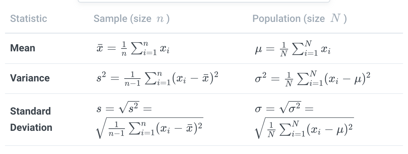
Make this table again with yellow text instead of using the image
A slight detour ... ...
Why do we square the deviations?
Make a single plot showing both |x-x_bar| and (x-x_bar)^2. the x-axis will be labeled as (x-x_bar) The data on x-axis will vary from -4 to 4
Reason1: The square function has better properties than the absolute function
Observation1: The square function is a smooth function and hence differentiable everywhere
Observation1: The absolute function is not differentiable at
Why do we square the deviations?
Reason1: The square function has better properties than the absolute function
Why do we care about differentiability?

In many applications (especially in ML) we need functions which are differentiable
Make a single plot showing both |x-x_bar| and (x-x_bar)^2. the x-axis will be labeled as (x-x_bar) The data on x-axis will vary from -4 to 4 (same a prev slide)
Why do we square the deviations?
Reason2: The square function magnify the contribution of outliers
Why do we want to magnify the contribution of outliers?

0.1, 0.2, 0.3, 0.3, 0.5, 0.1, 0.4, 0.2, 0.6, 10.2

Example: Toxic content in a fertiliser
What does the variance tell us about the data?
Variance: a measure of consistency
Alistair Cook: 2, 7, 7, 10, 14, 16, 37, 39, 244
Joe Root: 1, 9, 14, 15, 51, 58, 61, 67, 83
Ashes 2017-18 series (runs scored)
Mean = 39.88
Mean = 41.78
Does the variance capture this?

Observation: Root was more consistent than Cook
Variance: a measure of consistency
show two tables: showing the computation of variance and standard deviation for Root and Cook
framgments: one column at a time, quote

Indeed the lower variance shows that Root was more consistent than Cook
Variance: a measure of consistency

The primary objective of manufacturing industries is to ensure that there is little variance in their products
Desirable to have almost 0 variance in
length of sleeves
radius of tyres
weight of dumbbells
... ... ...
What is the effect of transformations on measures of spread
Transformations
Scaling and Shifting
(a = 5/9, c = -160/9)
[22.46, 23.54, 24.26, 27.86, 30.2, 30.74, 34.52, 35.96, 40.46, 44.06, 52.7, 54.68, 56.66, 57.56, 59.54, 61.52, 62.06, 65.66, 67.46, 70.88, 76.46, 82.4, 83.12, 84.38, 93.02, 94.28, 95.72, 96.44, 108.86, 109.58]
[-5.3, -4.7, -4.3, -2.3, -1.0, -0.7, 1.4, 2.2, 4.7, 6.7, 11.5, 12.6, 13.7, 14.2, 15.3, 16.4, 16.7, 18.7, 19.7, 21.6, 24.7, 28.0, 28.4, 29.1, 33.9, 34.6, 35.4, 35.8, 42.7, 43.1]
bad aesthetics
Effect of transformations (on range)
[22.46, 23.54, 24.26, 27.86, 30.2, 30.74, 34.52, 35.96, 40.46, 44.06, 52.7, 54.68, 56.66, 57.56, 59.54, 61.52, 62.06, 65.66, 67.46, 70.88, 76.46, 82.4, 83.12, 84.38, 93.02, 94.28, 95.72, 96.44, 108.86, 109.58]
[-5.3, -4.7, -4.3, -2.3, -1.0, -0.7, 1.4, 2.2, 4.7, 6.7, 11.5, 12.6, 13.7, 14.2, 15.3, 16.4, 16.7, 18.7, 19.7, 21.6, 24.7, 28.0, 28.4, 29.1, 33.9, 34.6, 35.4, 35.8, 42.7, 43.1]
Effect of transformations (on range)
bad aesthetics
Recap:
Effect of transformations (on IQR)
Effect of transformations (on IQR)
[22.46, 23.54, 24.26, 27.86, 30.2, 30.74, 34.52, 35.96, 40.46, 44.06, 52.7, 54.68, 56.66, 57.56, 59.54, 61.52, 62.06, 65.66, 67.46, 70.88, 76.46, 82.4, 83.12, 84.38, 93.02, 94.28, 95.72, 96.44, 108.86, 109.58]
[-5.3, -4.7, -4.3, -2.3, -1.0, -0.7, 1.4, 2.2, 4.7, 6.7, 11.5, 12.6, 13.7, 14.2, 15.3, 16.4, 16.7, 18.7, 19.7, 21.6, 24.7, 28.0, 28.4, 29.1, 33.9, 34.6, 35.4, 35.8, 42.7, 43.1]
compute the values of xx and yy
Exercise: Compute the first and third quartile for the transformed data and verify that the new IQR is indeed yy
bad aesthetics
Effect of transformations (on variance)
Effect of transformations (on std. dev.)
Effect of transformations (on variance)
[22.46, 23.54, 24.26, 27.86, 30.2, 30.74, 34.52, 35.96, 40.46, 44.06, 52.7, 54.68, 56.66, 57.56, 59.54, 61.52, 62.06, 65.66, 67.46, 70.88, 76.46, 82.4, 83.12, 84.38, 93.02, 94.28, 95.72, 96.44, 108.86, 109.58]
[-5.3, -4.7, -4.3, -2.3, -1.0, -0.7, 1.4, 2.2, 4.7, 6.7, 11.5, 12.6, 13.7, 14.2, 15.3, 16.4, 16.7, 18.7, 19.7, 21.6, 24.7, 28.0, 28.4, 29.1, 33.9, 34.6, 35.4, 35.8, 42.7, 43.1]
Exercise: Compute the variance and standard deviation for the original and transformed data and verify that:
bad aesthetics

Summary
Measures of centrality
Measures of spread
Effect of transformations
How do you use mean and variance to standardise data?
Standardising data
Question: How many standard deviations away from the mean is a given value x?
Intuition: Instead of expressing distances in absolute values, express them in units of standard deviations
Mean: 6.0 Std. dev: 2.97
1 2 3 4 5 6 7 8 9 10
-1 SD
-2 SD
+1 SD
+2 SD
We will have to change this example
In this example there is no data which is at +2,+3 or -2,-3 SD. Create a new example where there is some data at 2,3SD and -2,-3 SD and change the plot accordingly
Remember to divide by n-1 while computing the variance
Standardising data
If is the mean and s is the std. dev. then find the point which is one std. dev. away from the mean
what about 2 standard deviations?
what about z standard deviations?


Standardising data
We can express any point in the data as
where
is called the z-score and tells us the number of standard deviations that the point is away from the mean
We can express any point in the data as
Standardising data
for the data shown on slide 83 show a table showing the computation of z scores
The table will have two columns: x_i and z_i (give formula of z_i)
the mean and std. dev of the data at the bottom of the table
Standardising data (Usage in ML)
show a table with patient data containing 3 attributes: annual income (INR), weight (kg) and height (feet)
(a sample of 10 points)
write the range of each column below the column
Show an ML system which takes these 3 as inputs and predicts Health Risk/ No Risk (similar to a diagram that we used in one of the earlier lectures
Range:
| 2L | 65 | 5.8 |
| 5L | 60 | 5.5 |
| 10L | 75 | 6 |
| 8L | 70 | 5.3 |
| 4L | 54 | 5.2 |
| 7L | 60 | 5.3 |
| 1L | 50 | 5.3 |
| 20L | 72 | 6.2 |
| 7L | 82 | 6.1 |
| 3L | 67 | 5.9 |
20-1 = 19L
82-50 = 32Kgs
6.2-5.2 = 1.0ft
ML System
Income
Height
Weight
Health Risk
No Health Risk
Income (INR)
Height (Feet)
Weight (Kgs)
Standardising data (Usage in ML)
In addition to the table on the previous slide show a table where all the 3 columns are now in their standardised form
What is the mean and standard deviation of the standardised data?

| 2L | 65 | 5.8 |
| 5L | 60 | 5.5 |
| 10L | 75 | 6 |
| 8L | 70 | 5.3 |
| 4L | 54 | 5.2 |
| 7L | 60 | 5.3 |
| 1L | 50 | 5.3 |
| 20L | 72 | 6.2 |
| 7L | 82 | 6.1 |
| 3L | 67 | 5.9 |
| -0.86 | -0.05 | 0.37 |
| -0.31 | -0.56 | -0.42 |
| 0.6 | 0.97 | 0.89 |
| 0.24 | 0.46 | -0.95 |
| -0.49 | -1.18 | -1.21 |
| 0.05 | -0.56 | -0.95 |
| -1.04 | -1.59 | -0.95 |
| 2.44 | 0.66 | 1.42 |
| 0.05 | 1.69 | 1.16 |
| -0.68 | 0.15 | 0.63 |
Income (INR)
Height (Feet)
Weight (Kgs)
Income (INR)
Height (Feet)
Weight (Kgs)
Standardising data (Usage in ML)
What is the mean and standard deviation of the standardised data?

Is this always the case?

| -0.86 | -0.05 | 0.37 |
| -0.31 | -0.56 | -0.42 |
| 0.6 | 0.97 | 0.89 |
| 0.24 | 0.46 | -0.95 |
| -0.49 | -1.18 | -1.21 |
| 0.05 | -0.56 | -0.95 |
| -1.04 | -1.59 | -0.95 |
| 2.44 | 0.66 | 1.42 |
| 0.05 | 1.69 | 1.16 |
| -0.68 | 0.15 | 0.63 |
Mean: 0
Mean: 0
Mean: 0
Std: 0.9998
Std: 1
Std: 1
Income (INR)
Height (Feet)
Weight (Kgs)
Standardising data (Usage in ML)
Prove that the mean on the standardised data is 0
Proof:
Standardising data (Usage in ML)
Prove that the standard deviation of the standardised data is 1
Proof:
Summary (measures of spread)
Measures of spread
Except IQR all measures are sensitive to outliers
Measure of consistency in the data
Except variance, all measures have the same unit as the original data
Summary (measures of spread)
Effect of transformations
Standardising data

After standardising the data has zero mean and unit variance
What are box plots?
Box plots are used for visualising spread, median and outliers in the data

Box Plots
We say that x is an outlier if

or if
(a formal definition of outliers)
Box Plots
IQR
Median
Outliers
1.5 * IQR
1.5 * IQR
Box Plots
Shikhar Dhawan T20I scores (59 sorted scores)
0, 1, 1, 1, 1, 1, 2, 2, 3, 3, 3, 4, 5, 5, 5, 5, 6, 6, 8, 9, 10, 10, 11, 13, 14, 15, 16, 19, 23, 23, 23, 24, 26, 29, 30, 30, 31, 32, 32, 33, 35, 36, 40, 41, 41, 42, 43, 46, 47, 51, 52, 55, 60, 72, 74, 76, 80, 90, 92
Median = 23
Q1 = 5, Q3 = 41
IQR = 36
Q1 - 1.5 IQR = -49
Q3 + 1.5 IQR = 95
(no outliers on either side)
Box Plots
Median = 23
Q1 = 5, Q3 = 41
IQR = 36
Q1 - 1.5 IQR = -49
Q3 + 1.5 IQR = 95

Box Plots (Variant 1)
Median = 32
Q1 = 27.75, Q3 = 38.25
IQR = 10.5
Q1 - 1.5 IQR = 12
Q3 + 1.5 IQR = 54
max value = 45
choose some data which has at least few outliers only on one side
min value = 2
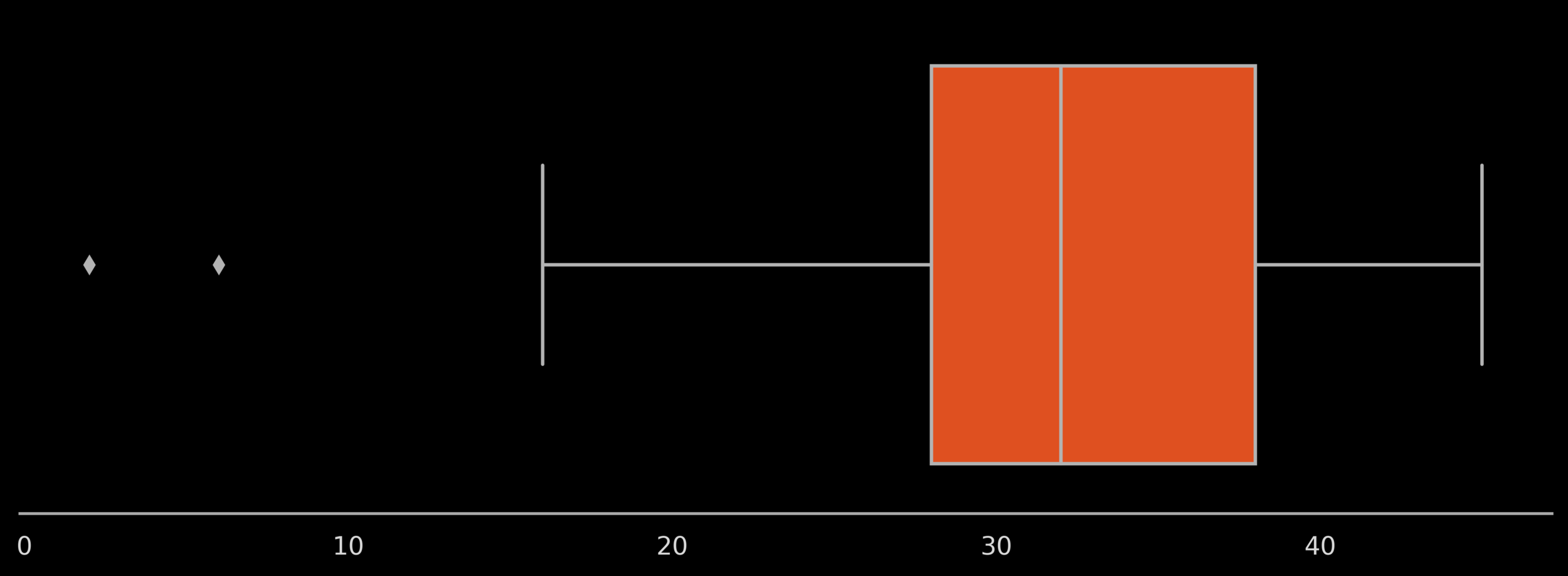
Box Plots (Variant 1)
Median = xx
Q1 = xx, Q3 = yy
IQR = zz
Q1 - 1.5 IQR = pp
Q3 + 1.5 IQR = rr
max value = 45
min value = 16
If there are no outliers move the whisker to the max/min value
plot corresponding to the data on the previous slide but matching the description of Variant1 in the gitbook
Box Plots (Variant 2)
choose same data as previous slide
Median = xx
Q1 = xx, Q3 = yy
IQR = zz
Q1 - 1.5 IQR = pp
Q3 + 1.5 IQR = rr
max value = zzzz
min value = zzzz
Box Plots (Variant 2)
five number summary: min, max, median, Q1, Q2
plot corresponding to the data on the previous slide but matching the description of Variant1 in the gitbook
also mark the 5 numbers on the plot
Median = xx
Q1 = xx, Q3 = yy
IQR = zz
Q1 - 1.5 IQR = pp
Q3 + 1.5 IQR = rr
max value = zzzz
min value = zzzz
Box Plots (Variant 3)
Median = xx
Q1 = xx, Q3 = yy
Q1 - 1.5 IQR = pp
Q3 + 1.5 IQR = rr
max value = zzzz (excluding outliers)
min value = zzzz (excluding outliers)
choose same data as previous slide
plot corresponding to the data on the previous slide but matching the description of Variant3 in the gitbook
Box Plots (Variant 3)
move the whisker to the max/min value obtained after excluding all outliers
Median = xx,
Q1 = xx, Q3 = yy
Q1 - 1.5 IQR = pp
Q3 + 1.5 IQR = rr
max value = zzzz (excluding outliers)
min value = zzzz (excluding outliers)
show box plot for left-skewed, right-skewed and symmetric data
the position of the median should be clearly highlighted in the plot
Box Plots: skewness in the data


show ML system for distinguishing between positive and negative reviews (we had such a diagram in one of the earlier lectures)
Box Plots (Usage in ML)
Evaluation:
(scores assigned by the system to + reviews)
(scores assigned by the system to - reviews)
ML System
or
Sample Review
Box Plots (Usage in ML)
Ideal box plot
(No overlap in the IQR of the scores assigned to positive and negative reviews)
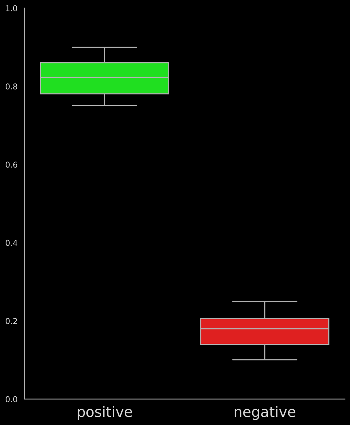
compare plots of five systems as given by Ananya
Box Plots (Usage in ML)
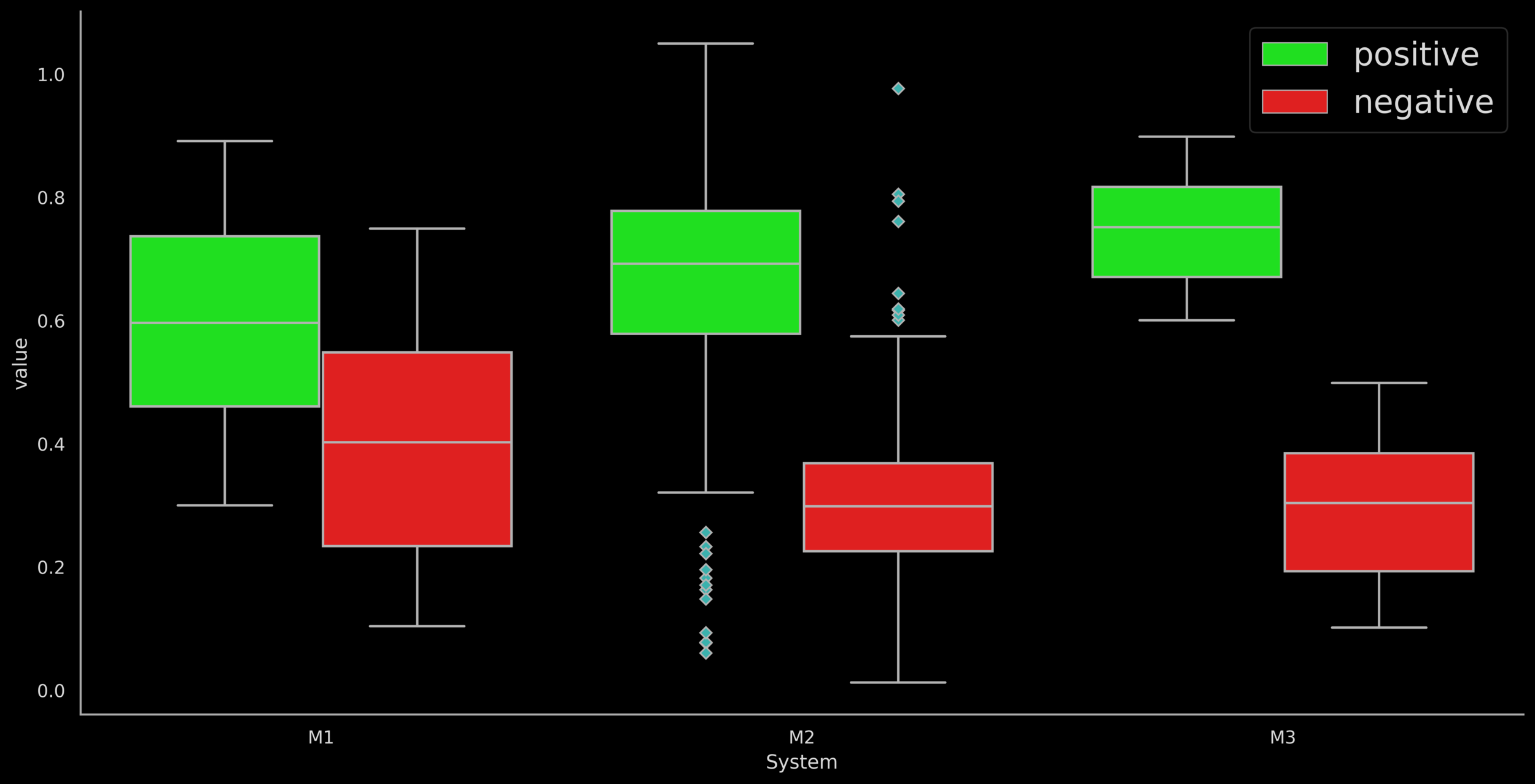
Box plots can be used to visually compare the performance of ML systems
- M1 does poorly, high overlap in IQRs of +ve and -ve
Ananya's notes: For comparing : (Please note that I have plotted for comparing 3 systems instead of 5 since I didn't have a description of M3 and M4 and felt adding those made the plot look more cluttered without much new information.)
- M2 does poorly, many outliers coinciding with opposite class IQR
- M3 does well in separating the +ve and -ve classes
Measures of Centrality
| Age | Height | Weight | Cholesterol | Sugar level | .... ..... |
|---|---|---|---|---|---|
| 32 | 165 | 75 | 124 | 108 | ... |
| 24 | 172 | 81 | 112 | 98 | ... |
| ... | ... | ... | ... | ... | ... |
| ... | ... | ... | ... | ... | ... |
| ... | ... | ... | ... | ... | ... |
Which is the 7th most grown crop in the country?
Hard to answer

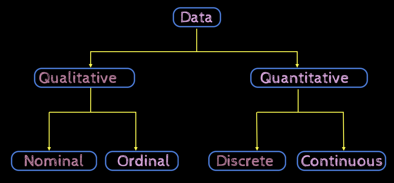
Nominal attributes


Recall
Question: What is the typical value of an attribute in our dataset?
How many runs does Sachin Tendulkar typically score in a match?


How many balls does Sachin Tendulkar typically face in a match?


Measures of Centrality
| Age | Height | Weight | Cholesterol | Sugar level | .... ..... |
|---|---|---|---|---|---|
| 32 | 165 | 75 | 124 | 108 | ... |
| 24 | 172 | 81 | 112 | 98 | ... |
| ... | ... | ... | ... | ... | ... |
| ... | ... | ... | ... | ... | ... |
| ... | ... | ... | ... | ... | ... |
Which is the 7th most grown crop in the country?
Hard to answer

Nominal attributes


Recall
Question: What is the typical value of an attribute in our dataset?
How many runs does Sachin Tendulkar typically score in a match?


How many balls does Sachin Tendulkar typically face in a match?

Motivation: Summarise Big Data
| Age | Height | Weight | Cholesterol | Sugar level | .... ..... |
|---|---|---|---|---|---|
| 32 | 165 | 75 | 124 | 108 | ... |
| 24 | 172 | 81 | 112 | 98 | ... |
| ... | ... | ... | ... | ... | ... |
| ... | ... | ... | ... | ... | ... |
| ... | ... | ... | ... | ... | ... |
Which is the 7th most grown crop in the country?
Hard to answer

Nominal attributes


ML System
or
Sample Review
Typically we feed words from the review to the ML system
Which words to give as input?
