Super-efficiency of automatic differentiation for functions defined as a minimum

https://arxiv.org/abs/2002.03722

Pierre Ablin$^1$, Gabriel Peyré$^1$, Thomas Moreau$^2$

1: ENS and CNRS, PSL university 2: Inria and CEA

Context

Sparse coding

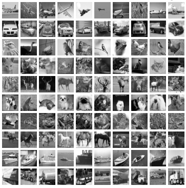
Let $k$ images $u_1, ..., u_k$ in $\mathbb{R}^d$.

$u_1, ..., u_k$ :

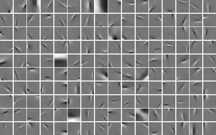
$D=[d_1, ...,d_m]$ a set of points in $\mathbb{R}^d$.

$D$ is the dictionary

$D =$

Sparse coding (contd)

Each image is decomposed in the basis of $D$:

$u_i \simeq z^i_1 d_1 +\cdots + z^i_m d_m$

$\simeq $

$3.1 \times$

$-1.4 \times$

$+ \cdots+0.6 \times$

$u_i$

$z^i_1 $

$z^i_2 $

$z^i_m $

$d_1$

$d_2$

$d_m$

$u_i \simeq Dz_i$

Sparse coding (contd)

$u_i \simeq Dz_i$

Sparse coding: $z$ should be sparse (many zeros). Estimated with the Lasso:

\min_{z\in\mathbb{R}^d} \mathcal{L}(z, D) =\frac12 \|u - Dz\|^2 + \lambda \|z\|_1

z^* = \argmin_z \mathcal{L}(z, D)

Dictionary learning

Instead of a fixed $D$, learn it from the data:

\ell(D) = \min_{z\in\mathbb{R}^d} \mathcal{L}(z, D)

D^* = \argmin \ell(D)

Double minimization problem !

We would like to do gradient descent on $D$.

How to compute the gradient of $\ell$?

Computing the gradient of a minimum

- Let $\mathcal{L}(z, x)$ a smooth function where $z\in \mathbb{R}^m$ and $x\in\mathbb{R}^n$, and

$$\boxed{\ell(x) = \min_z \mathcal{L}(z, x)}$$

- We want to compute $\nabla \ell(x)$

Examples: min-min optimization

- Dictionary learning

- Alternate optimization

- Frechet means

max-min optimization

- Game theory

- GANs

Technical assumptions

- $\ell(x) = \min_z \mathcal{L}(z, x)$, we want to compute $\nabla \ell(x)$

We assume:

- For all $x$, $\mathcal{L}$ has a unique minimizer $z^*(x)=\arg\min_z \mathcal{L}(z, x)$

$$\ell(x) = \mathcal{L}(z^*(x), x)$$

- $x\to z^*(x) $ is differentiable

Consequence (Danskin):

\nabla \ell(x) = \frac{\partial}{\partial x} \left[\mathcal{L}(z^*(x), x)\right]

\nabla \ell(x) = \frac{\partial z^*}{\partial x} \nabla_1\mathcal{L}(z^*(x), x) + \nabla_2 \mathcal{L}(z^*(x), x)

\boxed{\nabla \ell(x) = \nabla_2 \mathcal{L}(z^*(x), x)}

\nabla_1 \mathcal{L}(z^*(x), x) = 0

\nabla \ell(x) = \frac{\partial z^*}{\partial x} \underbrace{\nabla_1\mathcal{L}(z^*(x), x)}_{=0} + \nabla_2 \mathcal{L}(z^*(x), x)

Approximate optimization

- $\ell(x) = \min_z \mathcal{L}(z, x)$, we want to compute $\nabla \ell(x)$

-No closed-form: We assume that we only have access to a sequence $z_t$ such that $z_t \to z^*$

Example: $z_t$ produced by gradient descent on $\mathcal{L}$

- $z_0 = 0$

- $z_{t+1} = z_t - \rho \nabla_1 \mathcal{L}(z_t, x)$

- $z_t$ depends on $x$: $z_t(x)$

How can we approximate $\nabla \ell(x)$ using $z_t(x)$ ? At which speed ?

The analytic estimator

g^1_t(x) = \nabla_2 \mathcal{L}(z_t(x), x)

Very simple to compute: simply plug $z_t$ in $\nabla_2 \mathcal{L}$ !

\nabla \ell(x) = \nabla_2 \mathcal{L}(z^*(x), x)

z_t(x) \to z^*(x)

The automatic estimator

g^2_t(x) = \frac{\partial}{\partial x}\left[\mathcal{L}(z_t(x), x)\right]

$g^2_t$ is computed by automatic differentiation:

\nabla \ell(x) = \nabla_2 \mathcal{L}(z^*(x), x)

z_t(x) \to z^*(x)

g^2_t(x) = \frac{\partial z_t}{\partial x} \underbrace{\nabla_1\mathcal{L}(z_t(x), x)}_{\neq 0} + \nabla_2 \mathcal{L}(z_t(x), x)

- Easy to code (e.g. in Python, use pytorch, tensorflow, autograd...)

- $\sim$ as costly to compute as $z_t$

- Memory cost linear with # iterations

The implicit estimator

\nabla \ell(x) = \nabla_2 \mathcal{L}(z^*(x), x)

z_t(x) \to z^*(x)

Implicit function theorem:

\frac{\partial z^*(x)}{\partial x} = \mathcal{J}(z^*(x), x)

\mathcal{J}(z, x) = - \nabla_{21} \mathcal{L}(z, x)\left[\nabla_{11}\mathcal{L}(z, x)\right]^{-1}

g^3_t(x) = \mathcal{J}(z_t(x), x) \nabla_1\mathcal{L}(z_t(x), x) + \nabla_2 \mathcal{L}(z_t(x), x)

- Need to invert a linear system: might be too costly to compute

Three gradient estimators

\nabla \ell(x) = \nabla_2 \mathcal{L}(z^*(x), x)

z_t(x) \to z^*(x)

- Analytic: $g^1_t(x) = \nabla_2 \mathcal{L}(z_t(x), x)$

- Automatic: $g^2_t(x) = \frac{\partial z_t}{\partial x} \nabla_1\mathcal{L}(z_t(x), x) + \nabla_2 \mathcal{L}(z_t(x), x)$

- Implicit: $g^3_t(x) = \mathcal{J}(z_t(x), x) \nabla_1\mathcal{L}(z_t(x), x) + \nabla_2 \mathcal{L}(z_t(x), x)$

These estimators are all "consistent":

If $z_t(x)= z^*(x)$

\boxed{g^1_t(x) = g^2_t(x) = g^3_t(x) = \nabla \ell(x)}

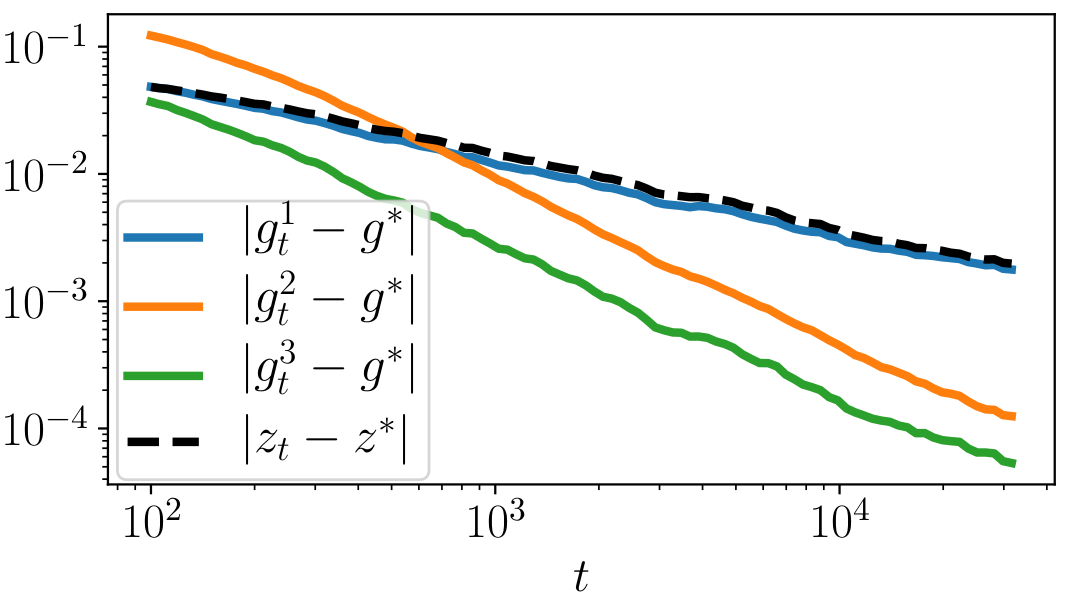
Convergence speed of the estimators

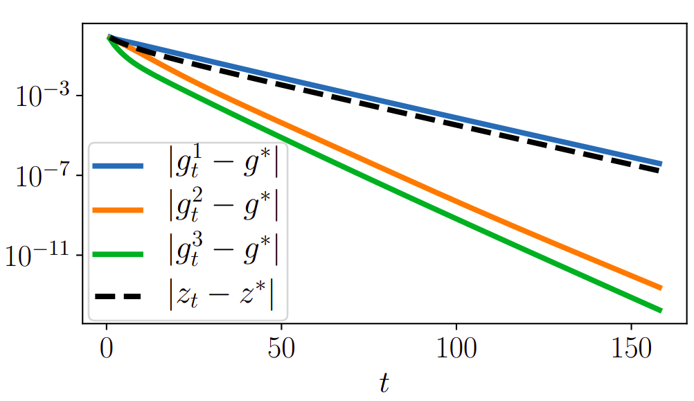
Toy example (regularized logistic regression)

$D$ rectangular matrix
$\mathcal{L}(z, x) = \sum_{i=1}^n\log\left(1 + \exp(-x_i[Dz]_i)\right) + \frac{\lambda}{2}\|z\|^2$
$z_t$ produced by gradient descent

Implicit estimator

g^1_t(x) = \nabla_2 \mathcal{L}(z_t(x), x)

If $\nabla_2 \mathcal{L} $ is $L$-Lipschitz:

|g^1_t(x) - \nabla \ell(x)| \leq L |z_t(x) - z^*(x)|

- The implicit estimator converges at the same speed as $z_t$

Automatic estimator

g^2_t(x) = \frac{\partial z_t}{\partial x} \nabla_1\mathcal{L}(z_t(x), x) + \nabla_2 \mathcal{L}(z_t(x), x)

It is of the form $g^2_t(x) = J \nabla_1 \mathcal{L}(z_t, x) + \nabla_2 \mathcal{L}(z_t, x)$, $J$ rectangular matrix

Taylor expansion around $z^*$:

\nabla_1\mathcal{L}(z_t, x) = \underbrace{\nabla_1 \mathcal{L}(z^*, x)}_{=0} + \left[\nabla_{11}\mathcal{L}(z^*, x)\right](z_t - z^*) + \underbrace{R_{11}}_{O(|z_t-z^*|^2)}

\nabla_1\mathcal{L}(z_t, x) = \left[\nabla_{11}\mathcal{L}(z^*, x)\right](z_t - z^*) + R_{11}

\nabla_2\mathcal{L}(z_t, x) = \underbrace{\nabla_2 \mathcal{L}(z^*, x)}_{\nabla\ell(x)} + \left[\nabla_{21}\mathcal{L}(z^*, x)\right](z_t - z^*) + \underbrace{R_{21}}_{O(|z_t-z^*|^2)}

\nabla_2\mathcal{L}(z_t, x) = \nabla\ell(x) + \left[\nabla_{21}\mathcal{L}(z^*, x)\right](z_t - z^*) + R_{21}

g^2_t(x) = \nabla \ell(x) + \underbrace{\left(J \nabla_{11}\mathcal{L}(z^*, x) + \nabla_{21}\mathcal{L}(z^*, x)\right)}_{R(J)}(z_t -z^*) + R_{21} + JR_{11}

g^2_t(x) = \nabla \ell(x) + R(J)(z_t - z^*) + O(|z_t-z^*|^2)

Automatic estimator

g^2_t(x) = \nabla \ell(x) + R(J)(z_t - z^*) + O(|z_t-z^*|^2), \text{ where } J = \frac{\partial z_t}{\partial x}

Implicit function theorem: $R(J) = J\nabla_{11}\mathcal{L}(z^*, x) + \nabla_{21}\mathcal{L}(z^*, x)$ cancels when $J = \frac{\partial z^*}{\partial x}$

If $\frac{\partial z_t}{\partial x} \to \frac{\partial z^*}{\partial x}$ then $R(J) \to 0$ and:

|g^2_t(x) -\nabla \ell(x) | = o(|z_t - z^*|)

Super-efficiency: Stricly faster than $g^1_t$ !

Implicit estimator

|g^3_t(x) -\nabla \ell(x) | =O(|z_t - z^*|^2)

Twice as fast as $g^1_t$ !

g^3_t(x) = \nabla \ell(x) + R(J)(z_t - z^*) + O(|z_t-z^*|^2)

\text{with } J = \mathcal{J}(z_t, x)= - \nabla_{21}\mathcal{L}(z_t, x)\left[\nabla_{11}\mathcal{L}(z_t, x)\right]^{-1}

If $\mathcal{J}$ is Lipschitz w.r.t. $z$:

Example

Gradient descent in the strongly convex case

Assumptions and reminders

-We assume that $\mathcal{L}$ is $\mu$-strongly convex and $L$-smooth w.r.t. $z$ for all $x$.

- $z_t$ produced by gradient descent with step $1/L$:

$z_{t+1} = z_t - \frac1L \nabla_1\mathcal{L}(z_t, x)$

Linear convergence:

\boxed{|z_t - z^*| \leq \kappa^t |z_0 - z^*|}\enspace, \enspace \kappa = (1 - \frac{\mu}{L})

Convergence of the Jacobian

$z_{t+1} = z_t - \frac1L \nabla_1\mathcal{L}(z_t, x)$

Let $J_t =\frac{\partial z_t}{\partial x}$ :

$J_{t+1} =J_t - \frac1L \left(J_t\nabla_{11}\mathcal{L}(z_t, x) + \nabla_{21}\mathcal{L}(z_t, x)\right) $

[Gilbert, 1992]:

\boxed{\|J_t - \frac{\partial z^*} {\partial x}\| = O(t\kappa^{t})}

Convergence speed of the estimators

\|J_t - \frac{\partial z^*} {\partial x}\| = O(t\kappa^{t})

|z_t - z^*\| = O(\kappa^{t})

|g^1_t(x)- \nabla\ell(x)| = O(\kappa^{t})

|g^2_t(x)- \nabla\ell(x)| = O(t\kappa^{2t})

|g^3_t(x)- \nabla\ell(x)| = O(\kappa^{2t})

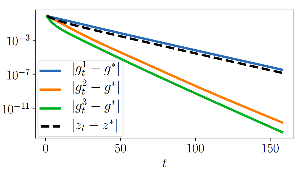
In the paper...

- Analysis in stochastic gradient descent case with step $\propto t^{-\alpha}$:

$|g^1_t - g^*| = O(t^{-\alpha})$, $|g^2_t - g^*| = O(t^{-2\alpha})$, $|g^3_t - g^*| = O(t^{-2\alpha})$

- Consequences on optimization: gradients are wrong, so what?

- Practical guidelines taking time and memory into account

Super-efficiency of automatic differentiation for functions defined as a minimum

Context

Sparse coding

Sparse coding (contd)

Sparse coding (contd)

Dictionary learning

Computing the gradient of a minimum

Technical assumptions

Approximate optimization

The analytic estimator

The automatic estimator

The implicit estimator

Three gradient estimators

Convergence speed of the estimators

Toy example (regularized logistic regression)

Implicit estimator

Automatic estimator

Automatic estimator

Implicit estimator

Example

Gradient descent in the strongly convex case

Assumptions and reminders

Convergence of the Jacobian

Convergence speed of the estimators

In the paper...

Thanks for you attention !