Approximate Bayesian Computation in Insurance
Patrick J. Laub and Pierre-Olivier Goffard

Just accepted to Insurance: Mathematics and Economics
Just pushed the package approxbayescomp to pip
Statistics with Likelihoods
For simple models we can write down the likelihood.
When simple rv's are combined, the resulting thing rarely has a tractable likelihood.
$$ X_1, X_2 \overset{\mathrm{i.i.d.}}{\sim} f_X(\,\cdot\,) \Rightarrow X_1 + X_2 \sim ~ \texttt{Intractable likelihood}! $$
Usually it's still possible to simulate these things...
Approximate Bayesian Computation
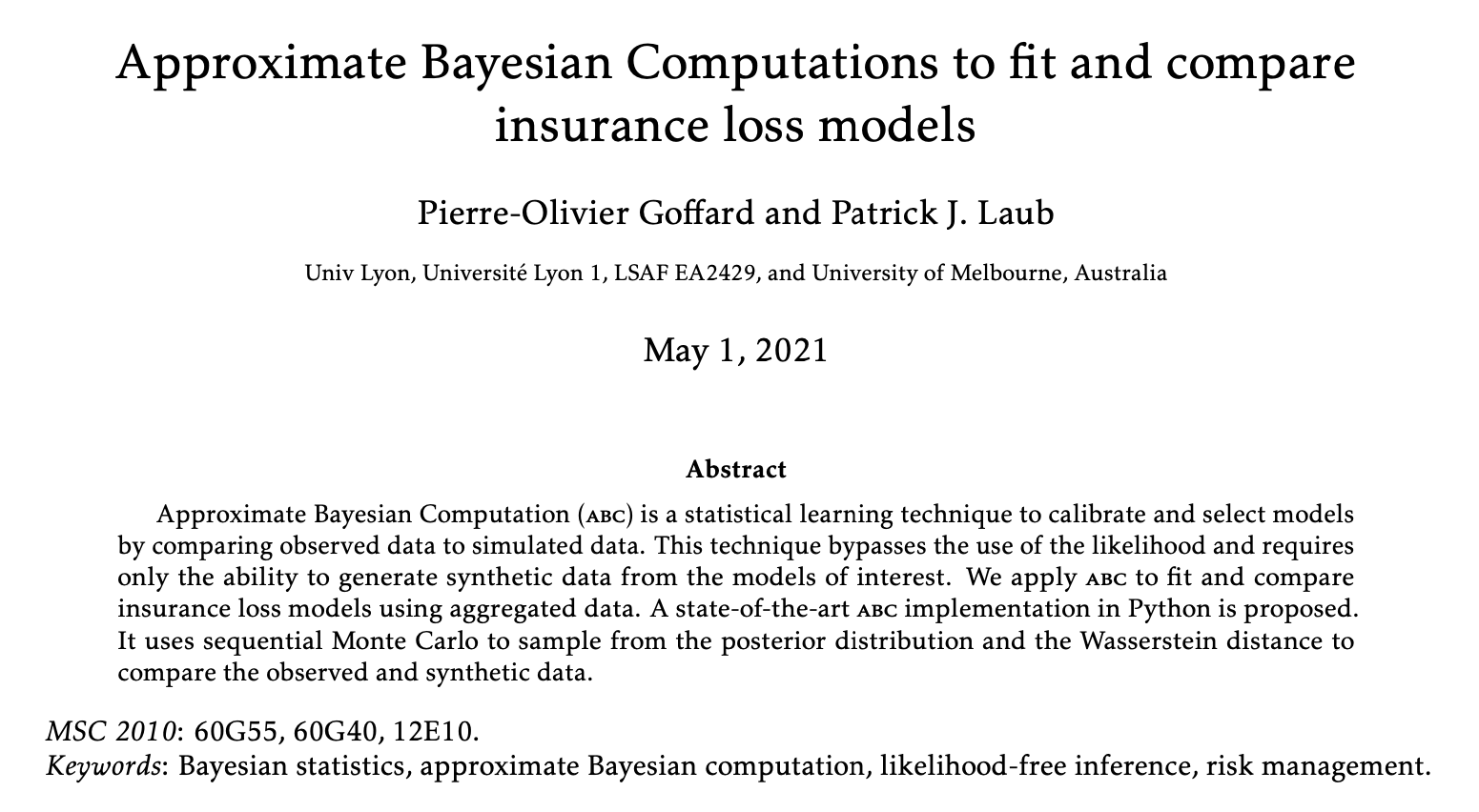
Example: Flip a coin a few times and get \((x_1, x_2, x_3) = (\text{H, T, H})\); what is
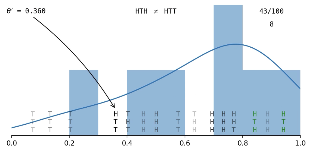
Getting an exact match of the data is hard...
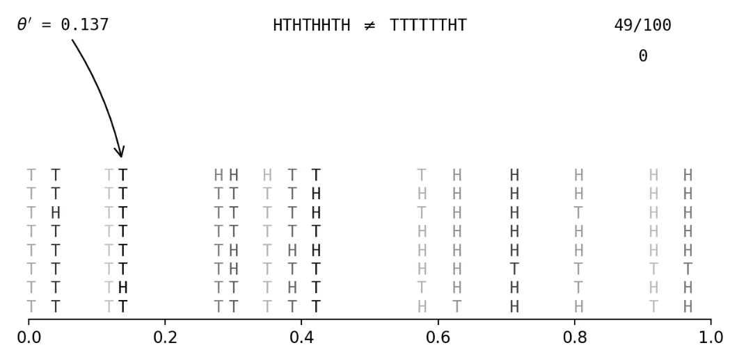
Accept fake data that's close to observed data
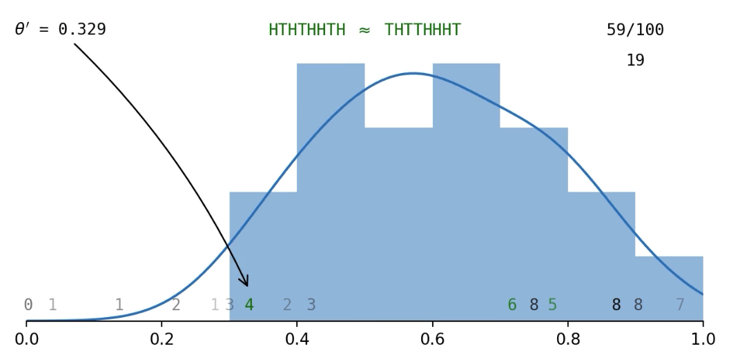
The 'approximate' part of ABC
Motivation
Have a random number of claims \(N \sim p_N( \,\cdot\, ; \boldsymbol{\theta}_{\mathrm{freq}} )\).
Random claim sizes \(U_1, \dots, U_N \sim f_U( \,\cdot\, ; \boldsymbol{\theta}_{\mathrm{sev}} )\).
We aggregate them somehow, like:
- aggregate claims: \(X = \sum_{i=1}^N U_i \)
- maximum claims: \(X = \max_{i=1}^N U_i \)
- stop-loss: \(X = ( \sum_{i=1}^N U_i - c )_+ \).
Question: Given a sample \(X_1, \dots, X_n\) of the summaries, what is the \(\boldsymbol{\theta} = (\boldsymbol{\theta}_{\mathrm{freq}}, \boldsymbol{\theta}_{\mathrm{sev}})\) which explains them?
E.g. a reinsurance contract
Does it work in theory?
Rubio and Johansen (2013), A simple approach to maximum intractable likelihood estimation, Electronic Journal of Statistics.
Proposition: Say we have continuous data \( \boldsymbol{x}_{\text{obs}} \) , and our prior \( \pi(\boldsymbol{\theta}) \) has bounded support.
If for some \(\epsilon > 0\) we have
$$ \sup\limits_{ (\boldsymbol{z}, \boldsymbol{\theta}) : \mathcal{D}(\boldsymbol{z}, \boldsymbol{x}_{\text{obs}} ) < \epsilon, \boldsymbol{\theta} \in \boldsymbol{ \Theta } } \pi( \boldsymbol{z} \mid \boldsymbol{ \theta }) < \infty $$
then for each \( \boldsymbol{\theta} \in \boldsymbol{\Theta} \)
$$ \lim_{\epsilon \to 0} \pi_\epsilon(\boldsymbol{\theta} \mid \boldsymbol{x}_{\text{obs}}) = \pi(\boldsymbol{\theta} \mid \boldsymbol{x}_{\text{obs}}) . $$
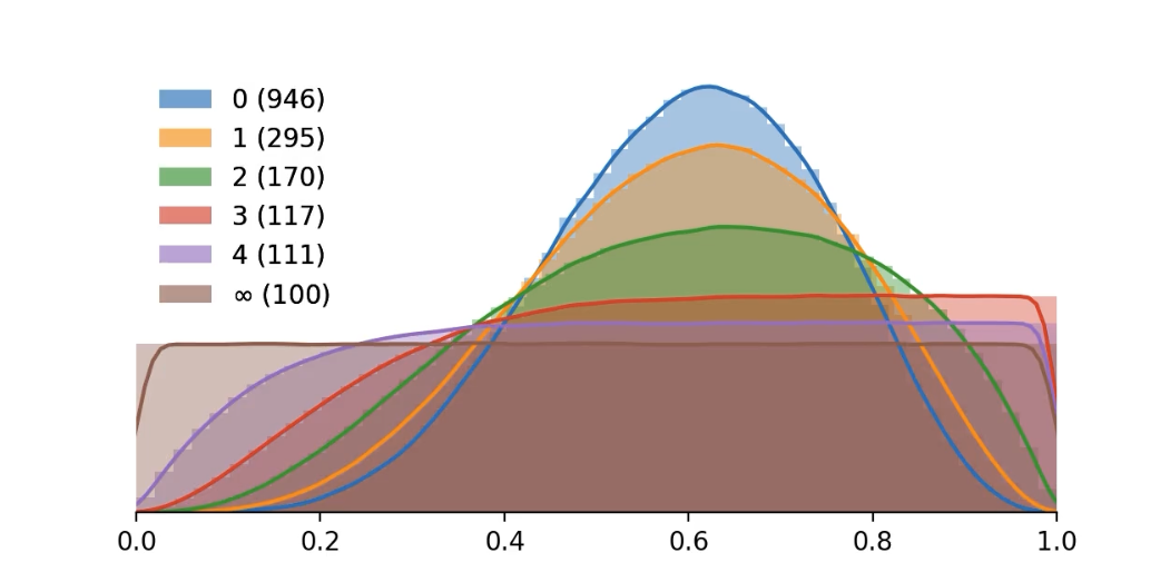
We sample the approximate / ABC posterior
$$ \pi_\epsilon(\boldsymbol{\theta} \mid \boldsymbol{x}_{\text{obs}}) \propto \pi(\theta) \times \mathbb{P}\bigl( \lVert \boldsymbol{x}_{\text{obs}}-\boldsymbol{x}^{\ast} \rVert \leq \epsilon \text{ where } \boldsymbol{x}^{\ast} \sim \boldsymbol{\theta} \bigr) , $$
but we care about the true posterior \( \pi(\boldsymbol{\theta} \mid \boldsymbol{x}_{\text{obs}}) \) .
Mixed data
Get
$$ \lim_{\epsilon \to 0} \pi_\epsilon(\boldsymbol{\theta} \mid \boldsymbol{x}_{\text{obs}}) = \pi(\boldsymbol{\theta} \mid \boldsymbol{x}_{\text{obs}}) $$
when
We filled in some of the blanks for mixed data.
Our data was mostly continuous data but had an atom at 0.
Does it work in practice?
Examples on simulated data
Dependent example
J. Garrido, C. Genest, and J. Schulz (2016), Generalized linear models for dependent frequency and severity of insurance claims, IME.
-
frequency \(N \sim \mathsf{Poisson}(\lambda=4)\),
-
severity \(U_i \mid N \sim \mathsf{DepExp}(\beta=2, \delta=0.2)\), defined as \( U_i \mid N \sim \mathsf{Exp}(\beta\times \mathrm{e}^{\delta N}), \)
-
summation summary \(X = \sum_{i=1}^N U_i \)
ABC posteriors based on 50 \(X\)'s and on 250 \(X\)'s given uniform priors.

Time-varying example
- Claims form a Poisson process point with arrival rate \( \lambda(t) = a+b[1+\sin(2\pi c t)] \).
- The observations are \( X_s = \sum_{i = N_{s-1}}^{N_{s}}U_i \).
- Frequencies are \(\mathsf{CPoisson}(a=1,b=5,c=\frac{1}{50})\) and sizes are \(U_i \sim \mathsf{Lognormal}(\mu=0, \sigma=0.5)\).


- Claims form a Poisson process point with arrival rate \( \lambda(t) = a+b[1+\sin(2\pi c t)] \).
- The observations are \( X_s = \sum_{i = N_{s-1}}^{N_{s}}U_i \).
- Frequencies are \(\mathsf{CPoisson}(a=1,b=5,c=\frac{1}{50})\) and sizes are \(U_i \sim \mathsf{Lognormal}(\mu=0, \sigma=0.5)\).
- ABC posteriors based on 50 \(X\)'s and on 250 \(X\)'s with uniform priors.

Time-varying example

From the same \( \boldsymbol{\theta} \) the data is random
Bivariate example
- Two lines of business with dependence in the claim frequencies.
- Say \( \Lambda_i \sim \mathsf{Lognormal}(\mu \equiv 0, \sigma = 0.2) \).
- Claim frequencies \( N_i \sim \mathsf{Poisson}(\Lambda_i w_1) \) and \( M_i \sim \mathsf{Poisson}(\Lambda_i w_2) \) for \(w_1 = 15\), \(w_2 = 5\).
- Claim sizes for each line are \(\mathsf{Exp}(m_1 = 10) \) and \(\mathsf{Exp}(m_2 = 40)\).
- ABC posteriors based on 50 \(X\)'s and on 250 \(X\)'s with uniform priors.


Streftaris and Worton (2008), Efficient and accurate approximate Bayesian inference with an application to insurance data, Computational Statistics & Data Analysis
ABC turns a statistics problem into a programming problem
... to be used as a last resort
import approxbayescomp as abc

# Load data to fit
obsData = ...

# Frequency-Loss Model
freq = "poisson"
sev = "frequency dependent exponential"
psi = abc.Psi("sum") # Aggregation process

# Fit the model to the data using ABC
prior = abc.IndependentUniformPrior([(0, 10), (0, 20), (-1, 1)])
model = abc.Model(freq, sev, psi, prior)
fit = abc.smc(numIters, popSize, obsData, model)
pip install approxbayescomp
Compiled code
(use numba)
Interpreted vs compiled code
C.f. Lin Clark (2017), A crash course in JIT compilers


def sample_geometric_exponential_sums(T, p, μ):
  X = np.zeros(T)

  N = rnd.geometric(p, size=T)
  U = rnd.exponential(μ, size=N.sum())

  i = 0
  for t in range(T):
    X[t] = U[i:i+N[t]].sum()
    i += N[t]

  return X
Interpreted version
from numba import njit

@njit()
def sample_geometric_exponential_sums(T, p, μ):
  X = np.zeros(T)

  N = rnd.geometric(p, size=T)
  U = rnd.exponential(μ, size=N.sum())

  i = 0
  for t in range(T):
    X[t] = U[i:i+N[t]].sum()
    i += N[t]

  return X
First run is compiling (500 ms), but after we are
down from 2.7 ms to 164 μs (16x speedup)
Compiled by numba
Original code: 1.7 s
Basic profiling with snakeviz: 5.5 ms, 310x speedup
+ Vectorisation/preallocation with numpy: 2.7 ms, 630x speedup
+ Compilation with numba: 164 μs, 10,000x speedup
And potentially:
+ Parallel over 80 cores: say another 50x improvement,
so overall 50,000x speedup.
Take-home messages
- What is ABC?
- Check out the paper on arXiv (see https://pat-laub.github.io)
- Install the package: pip install approxbayescomp