Bouncing universe: possibilities and challenges
PHY663 Term Paper Presentation
Prajakta Mane
MS19054
The Horizon Problem
WHY?
The difficulty in explaining the observed homogeneity of causally disconnected regions of space in the absence of a mechanism that sets the same initial conditions everywhere.
The observations of the cosmic microwave background (CMB) and galaxy surveys show that the observable universe is nearly isotropic and homogeneous. The temperatures of the CMB are coordinated to a level of . This suggests that the entire observable universe must have been causally connected long enough for the universe to come into thermal equilibrium.
Proposed solutions: cosmic inflation, a bouncing universe, a variable speed of light.
Inflation and perturbations
1. Inflation provides a way for particles that are not causally connected today to be causally connected in the past.
2. Also accounts for the origin of perturbations.
3. During inflation, Hubble radius suddenly decreases to allow 1, implying that . This accelerating expansion of universe requires the pressure of the sourcing field to be negative.
4. Theoretical scalar field sourcing inflation with negative pressure, having more potential energy density than kinetic.
5. Solving tensor and scalar perturbation modes in this setting,
Bouncing universe scenarios:
1. Matter bounce scenario
2. Pre-Big-Bang Scenario
3. Ekpyrotic Scenario
4. String Gas Cosmology
Matter Bounce:
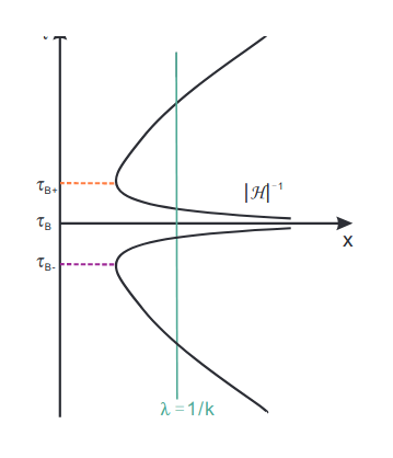
An initial matter-dominated phase of contraction during which scales that are currently probed with cosmological observations exit the Hubble radius.
Fixed comoving scales start out with a wavelength smaller than the Hubble radius, thus making a causal generation
mechanism for fluctuations possible.
1. The particle horizon is infinite since time extends to −∞. The entire spatial surface at the time of recombination in the CMB is within the causal horizon.
2. Leads to scale-invariant power spectrum.
Actuation of a bouncing phase
1. Modified matter (Einstein's GR +a modified matter component that is allowed to have negative energy density):
Introduce a “ghost” field (opposite side KE) whose energy density grows relative to that of regular matter during the contraction phase. For example, the regular matter can be described by a perfect fluid or by a massive scalar φ field whose time-averaged energy density scales as 1/a^3, and ghost matter by a free scalar field ψ with opposite sign kinetic term whose energy density is dominated by the ̇ψ2 term and whose energy density hence scales as 1/a^6. The non-singular bounce takes place when the energy densities of φ and ψ become equal.
2. Modified gravity
3. Superstring theory
Observational Signatures
Non-gaussianities:
Bouncing models contain many interaction terms so that the bounce and the previous phases take place which lead to an extra contribution to the 3-point corelation function.
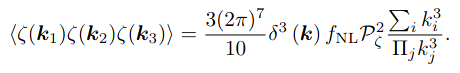
Many models of bouncing cosmology predict large contributions to these non-Gaussianties. In a bouncing model, just as in inflation, perturbations and non-Gaussianities are produced at Hubble crossing. Although the subsequent evolution of the non-Gaussianities might be different because:
1. During the initial contraction phase, the modes may change with time, producing a more important growth, leading to larger contribution of non-Gaussianities.
2. Existence of the bounce has a tendency to increase any pre-existing non-
Gaussianity.
Observational Signatures
Running of the scalar spectrum
Simple single field inflationary models give the red tilt of the scalar spectrum as the Hubble expansion rate H is very slowly decreasing during the period of inflation, which gives the negative slope of the power spectrum. This is the negative 'running' of the spectrum.
In the matter bounce case, the tilt of the spectrum of cosmological perturbations is caused by the fact that the contribution of the dark energy component is decreasing as a function of time during the contracting phase. This implies that at large values of k, the spectrum converges to a scale-invariant one, and
that thus the running of the scalar spectrum is positive.
Thus, a measurement of the running of the scalar spectrum would allow us to differentiate the canonical single field inflation models from the matter bounce scenario.
Observational Signatures
Tensor to scalar ratio
Before the bounce: O(1).
During the bounce: scalar modes might get enhanced compared to the tensor modes, leading to large r.
Does not provide a good differentiator between matter bounce and inflation.
Challenges:
Cosmology Standard model problems:
Horizon problem: time runs from −∞, the horizon can be infinite, explains horizon problem.
Flatness problem: symmetric matter bounce leads to a decrease in the curvature energy by the same amount that it increases during inflation.
Entropy problem: The universe starts large and cold in the matter-bounce universe implying that the entropy problem does not remain in the bouncing universe theory.
Initial conditions problem:
In any cosmological model, it is necessary to specify initial conditions. In a successful early universe model the initial conditions should not have to be finely tuned. Models of bouncing cosmologies must impose initial conditions at a time as far remote in the past as possible, and this corresponds to a moment when the Universe was large and mostly empty. All relevant scales are then inside the Hubble radius at the time the initial conditions are set up. Given the cosmological background, it is hence natural to assume quantum vacuum initial conditions for the fluctuations. On the other hand it is not so easy to justify the initial conditions for the background
Challenges:
Initial inhomogeneity:
In the matter bounce scenario, if the contraction sufficiently slow compared to the diffusion rate of the primordial constituents, an initially large contracting dust-dominated universe can wipe out any primordial inhomogeneity and yield a satisfactory initial state out of which one can settle vacuum initial conditions leading to our
universe. Although in this framework, in the contracting phase, presence of a cosmological constant could easily destabilize the perturbations, leading to predictions in disagreement with the current data.
Instabilities
Scalar and vector perturbations can grow too large leading to instabilities after the bounce.
References:
1. Brandenberger, R., Peter, P. Bouncing Cosmologies: Progress and Problems. Found Phys 47, 797–850 (2017). https://doi.org/10.1007/s10701-016-0057-0
2. Scott Dodelson, "Modern Cosmology" (2003): Chapter 6.
3. R. H. Brandenberger, “The Matter Bounce Alternative to Inflationary Cosmology,” arXiv:1206.4196 [astro-ph.CO].
4. R. H. Brandenberger, “Lectures on the theory of cosmological perturbations,” Lect. Notes Phys. 646, 127(2004) [arXiv:hep-th/0306071].
5. M. Novello and S. E. P. Bergliaffa, “Bouncing Cosmologies,” Phys. Rept. 463, 127 (2008)
doi:10.1016/j.physrep.2008.04.006 [arXiv:0802.1634 [astro-ph]].