

Prateek Narang & Mohit Uniyal

- Machine Learning vs Artificial Intelligence
- ML vs DL vs AI
- Computer Vision
- Natural Language Processing
ML & AI Introduction

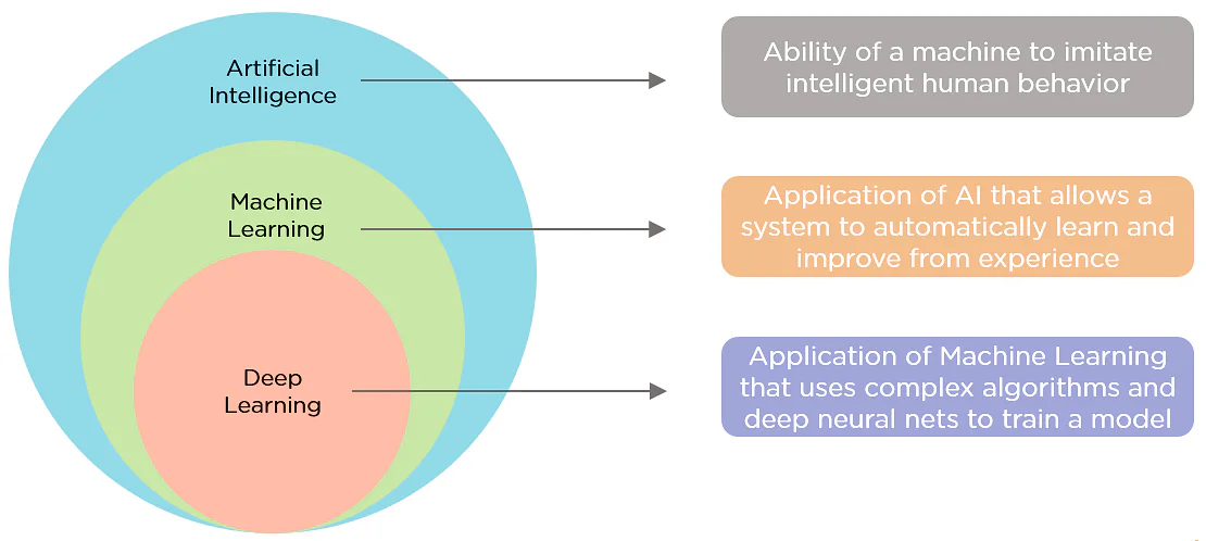
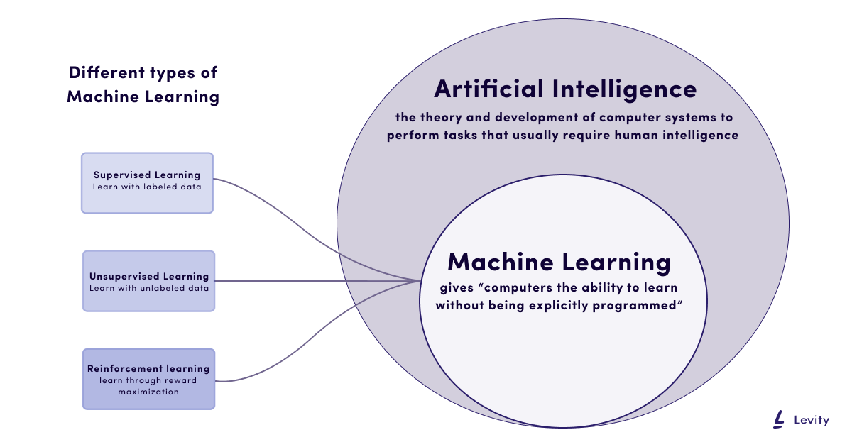
Artificial Intelligence vs Machine Learning vs Deep Learning
Buzzwords!
Subfields in Artificial Intelligence
1. Machine Learning (ML)
2. Deep Learning (DL)
3. Computer Vision (CV)
4. Natural Language Processing (NLP)
5. Automatic Speech Recognition (ASR)
6. Reinforcement Learning (RL)
- Machine learning covers a range of statistical techniques giving computers the ability to learn from data.
-
Create a statistical model to mimic “Intelligent” decision making.
-
Finding patterns in complex, scattered data to present information.
There are more than a dozen of these statistical techniques, one of which is deep learning.
1. Machine Learning
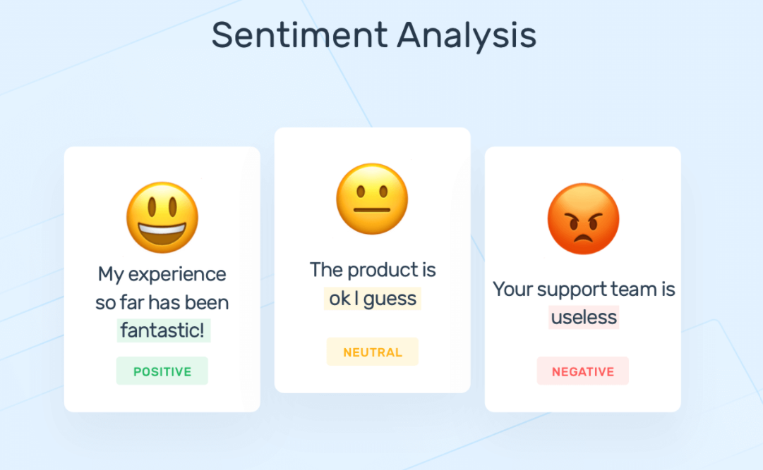
Model that identifies the sentiment of the text
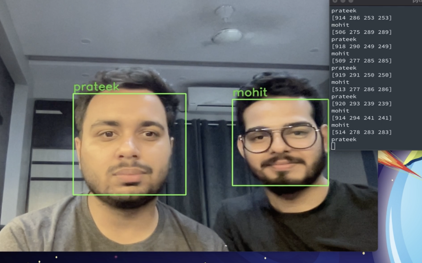
Model that classifies the the person in the image
Model that predicts the price of the house from historic data

Machine Learning algorithms is further subdivided into 3 subareas/paradigms :
- Supervised Learning
- Unsupervised Learning
- Reinforcement Learning
2. Deep Learning
-
Deep learning using artificial neural networks which are more complex models and can be trained for specific tasks.
-
Deep Learning models are data hungry and are more computationally expensive.
Deep learning models are often used in Computer Vision and Natural Language Processing.
Image Classifier

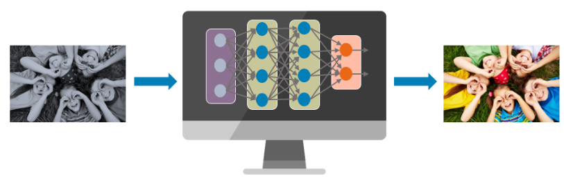
Image Colorisation
Image colorization has seen significant advancements using Deep Learning. ChromaGAN is an example of a picture colorization model.
Automatic Machine Translation
Language translation is supported by seq-2-seq models.

3. Computer Vision
-
Computer vision is an interdisciplinary field concerning how computers can see and understand digital images and videos.
-
Examples - Facial Recognition, Image Segmentation, Object Detection
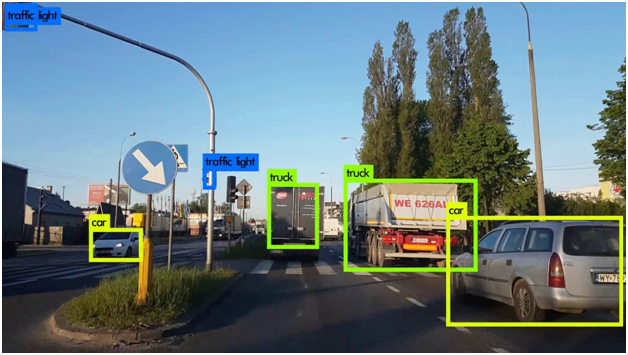
Detecting Objects in a scene
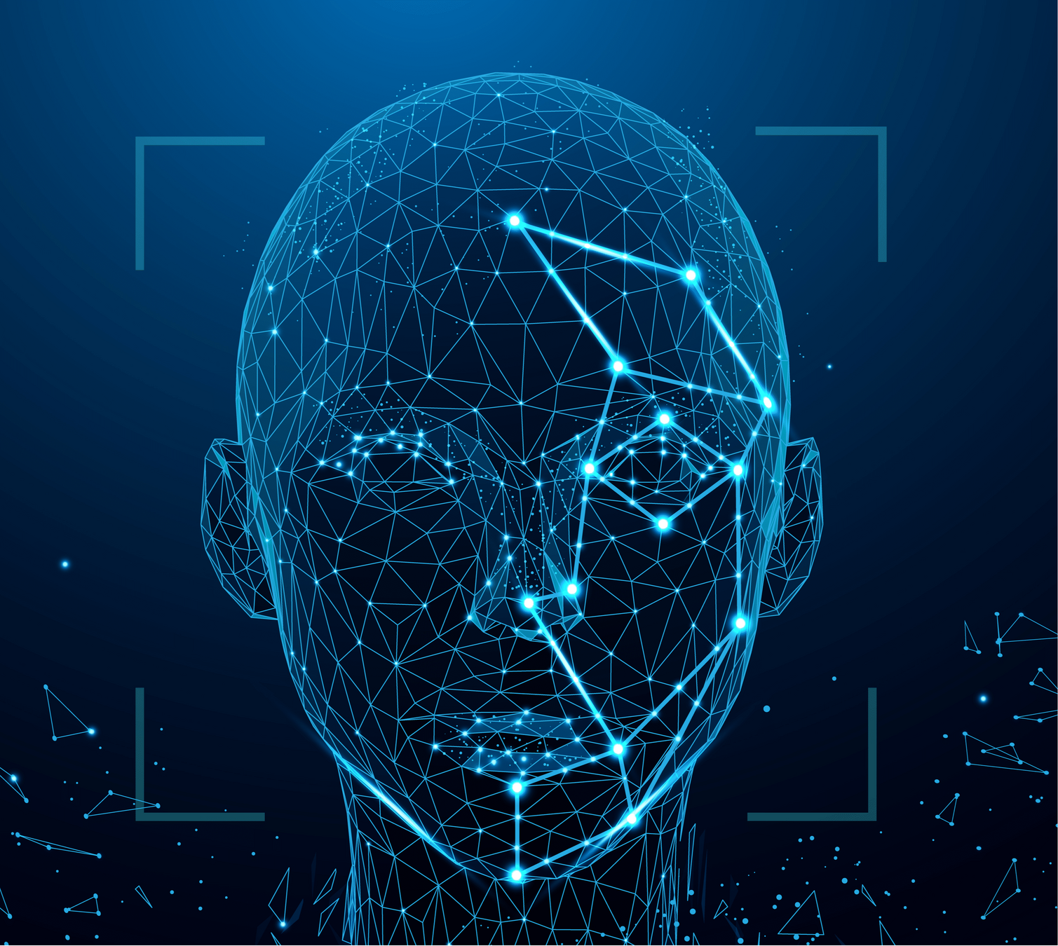
Facial Recognition on iPhone
4. Natural Language Processing
Natural-language processing (NLP) deals with the interactions between computers and human (natural) languages.
NLP separates into 2 sub-categories:
1) Natural-language understanding
2) Natural-language generation
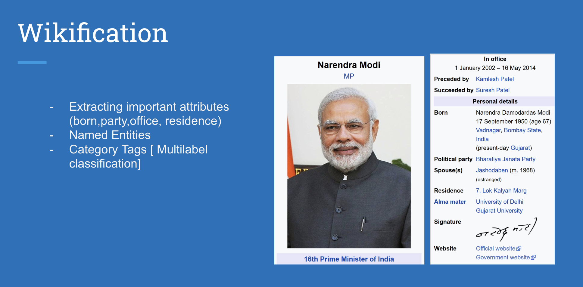
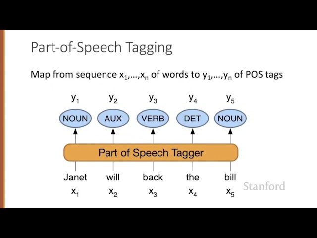
Named Entity Recognition

Chatbots like ChatGPT, Google Bard
5. Automatic Speech Recognition (ASR)
Automatic Speech Recognition allows human beings to use their voices to speak with a computer interface in a way that, in its most sophisticated variations, resembles normal human conversation.
Imagine you are late for a meeting and you need to send a message to your friend, so you open your phone,
click Dictation, say “Hi Prateek, I’m on my way” and click send.

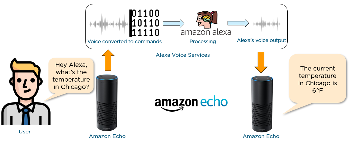
Amazon Alexa
Summary
- NLP is concerned with the meaning of words.
- Computer vision is concerned with recognising images and videos.
- ASR is concerned with the meaning of sounds.
Machine Learning is common in all of them!
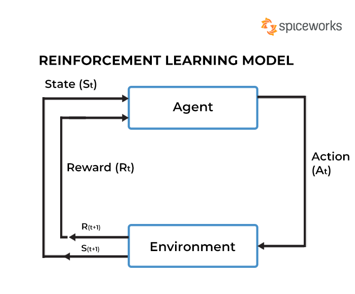
6. Reinforcement Learning
The goal of reinforcement learning is to train an agent to complete a task within an uncertain environment.
The agent receives observations and a reward from the environment and sends actions to the environment.
The reward measures how successful action is with respect to completing the task goal.

Learning to drive a bicycle!
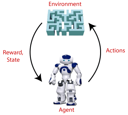
Autonomous robots
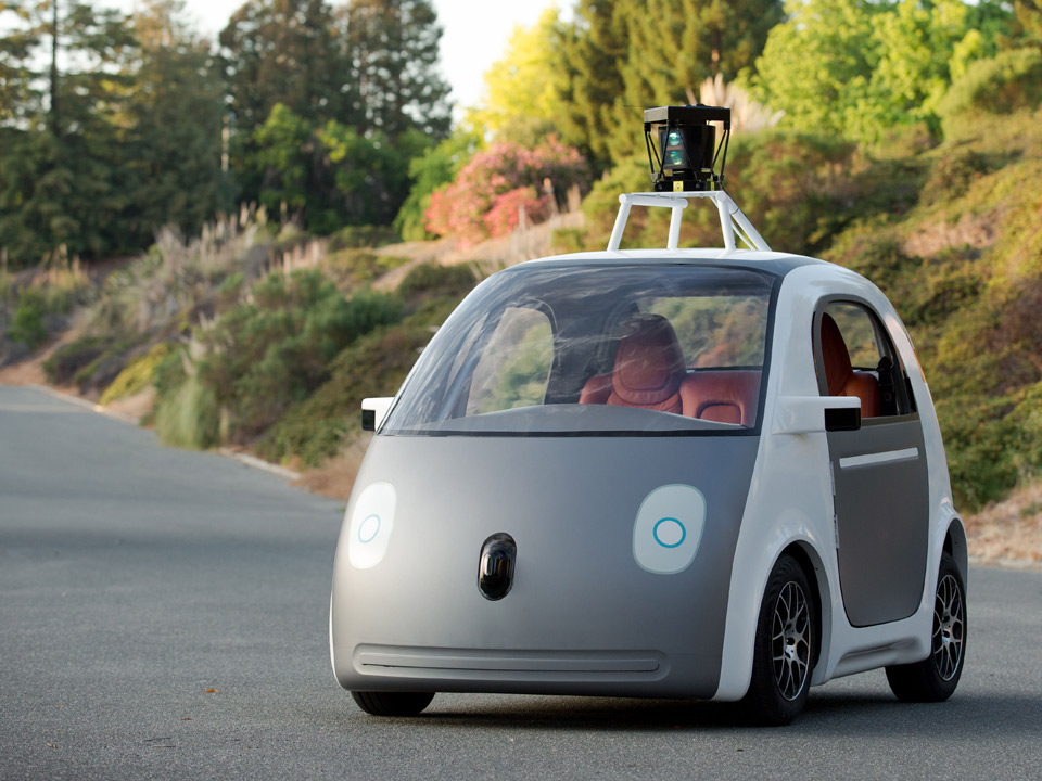
Self Driven Cars
Understand & implement popular machine learning algorithms and solve real-life problems
Machine Learning Essentials

Prateek Narang
Ex-Software Engineer, Instructor,
Co-Founder Coding Minutes
Mohit Uniyal
Data Scientist, Instructor,
Co-Founder Coding Minutes
Mentor at Google Code-In
Machine Learning is everywhere!
-
Conversation engines like ChatGPT
-
Medical Diagnosis
-
Apps like Google Photos, Youtube, News, Snapchat filters
-
Facebooks & Google Ads
-
Surveillance Systems
-
Self-driven cars
-
Generative AI - can create pictures, poems, essays
-
Recommender Systems - Netflix, Amazon, Youtube
-
Weather forecasting
-
Photography - Night Mode
-
Smart Devices - Amazon Alexa, Google Home

- Supervised Learning
- Regression
- Classification
- Text
- Images
- Numeric Data
- Unsupervised Learning
- Clustering
- Dimensionality Reduction
Fundamental Machine Learning Problems
ML Techniques from scratch!
Understand the maths and implement all algorithms from scratch and later with sci-kit learn.
- Linear Regression
- Logistic Regression
- Principal Component Analysis
- Naive Bayes
- Decision Trees
- Bagging and Boosting
- K-NN
- K-Means
- Neural Networks


- Convex Optimisation
- Overfitting vs Underfitting
- Bias Variance Tradeoff
- Performance Metrics
- Data Pre-processing
- Feature Engineering
- Working with numeric data, images & textual data
- Parametric vs Non-Parametric Techniques
Machine Learning Concepts
8+ Projects!
- Completely hands-on
- End to end coding
- Learn skills like
- Working with OpenCV
- Working with NLTK
- Filling Missing values
- Data Pre-processing

- House Price Prediction
- Digit Classification
- Face Recognition
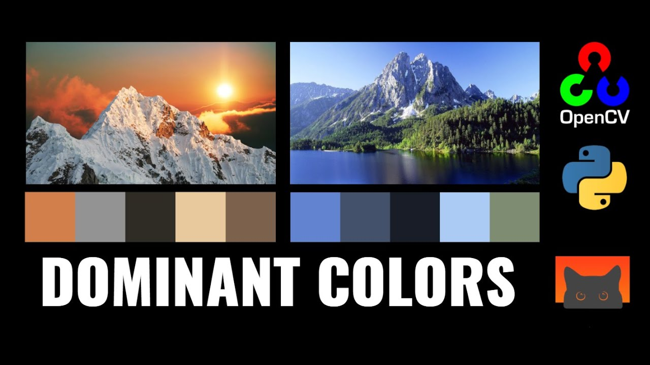
- Dominant Color Extraction
- Spam / Text Classification
- Titanic Survival Prediction
- Customer Churn Prediction
- Image Classification

Course Projects
Who can join?
Designed for beginners and curious learners, who really want to understand in's and out's of Machine Learning techniques and build a solid foundation for a data science career.
Proficiency in python is recommended for this course.

Thank you!
Looking forward to see you in the course!

- Supervised Learning
- Regression
- Classification
- Problems
- Code
Supervised Learning

Supervised Learning
In supervised learning, we use labeled datasets (training examples and their associated correct labels) to train algorithms that to classify data or predict outcomes accurately.
Regression and Classification are two tasks of supervised learning.


Regression: Predict a continuous numerical value. How much will that house sell for?
Classification: Assign a label. Is this a picture of a cat or a dog?
Regression vs Classification

Example
Let's examine the problem of predicting student's marks based upon number of hours someone has put in studying before the exam.
| Time Spent (X) | Marks (Y) |
|---|---|
| 5 | 16 |
| 3 | 10 |
| 4 | 13 |
| 11 | 34 |
Training Examples
Text
Data
The data is split into a training data set and a test data set.
The training set has labels, so your model can learn from these labeled examples.
The test set does not have labels, i.e. you don’t yet know the value you’re trying to predict.
It’s important that your model can generalize to situations it hasn’t encountered before so that it can perform well on the test data
| Time Spent (X) | Marks (Y) |
|---|---|
| 5 | 16 |
| 3 | 10 |
| 4 | 13 |
| 11 | 34 |
Training Examples
| Time Spent (X) | Predicted Marks |
|---|---|
| 6 | |
| 12 | |
| 2 | |
| 8 |
Test Examples
| Time Spent (X) | Marks (Y) |
|---|---|
| 5 | 16 |
| 3 | 9.8 |
| 4 | 13.5 |
| 11 | 34 |
More realistic data!
Training Examples
In a more formal way, we would like to build a model that approximates the relationship f between number of hours X and marks scored Y.
X (input) - number of hours of study
Y(output) - marks scored
f (function) - describing the relationship b/w X and Y
ε (espsilon) - random error with zero mean to account for unmodeled features/ inherent noise in the data
In supervised learning, the machine attempts to learn the relationship between X and Y, by running labeled training data through a learning algorithm
Training Examples (X,Y)
Learning Algorithm
Training Examples (X,Y)
f (hypothesis function)
Xtest
Ypred
- Linear Regression
- Error Function
- Gradient Descent
- Implementation
- Evaluation
- House Price Challenge
Linear Regression

Linear Regression
(also known Ordinary Least Squares)
Regression predicts a continuous value.
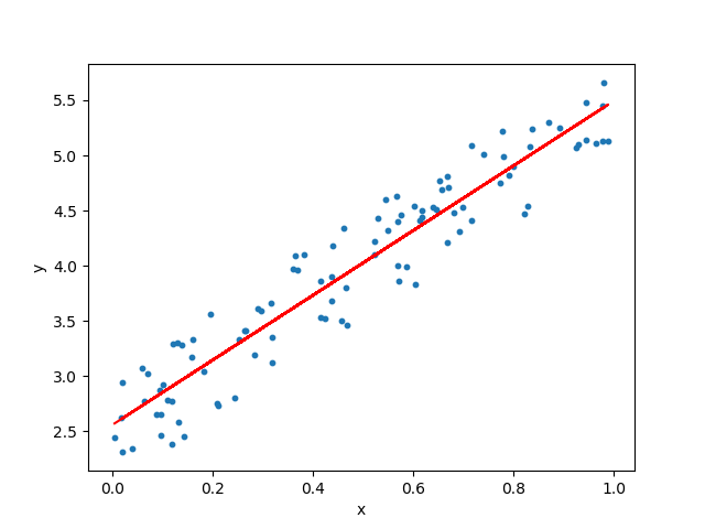
Now we will build an algorithm that solves the task of predicting marks given a labelled dataset.
The goal of the algorithm is to learn a linear model that predicts a y for an unseen x with minimum error.
| Time Spent (X) | Marks (Y) |
|---|---|
| 5 | 16 |
| 3 | 9.8 |
| 4 | 13.5 |
| 11 | 34 |
| ... | ... |
| Time Spent (X) | Marks (Y) |
|---|---|
| 5 | 12 |
| 3 | 8 |
| 4 | 10 |
| 11 | 24 |
| Time Spent (X) | Predict Marks (Y) |
|---|---|
| 6 | __ |
| 9 | __ |
| 10 | __ |
| 14 | ___ |
Notation
| Time Spent (X) | Marks (Y) |
|---|---|
| 5 | 16 |
| 3 | 9.8 |
| 4 | 13.5 |
| 11 | 34 |
| ... | ... |
n→number of featuresm→number of training examplesX→input data matrix of shape (mxn)y→ target value (can be a Real number)x(i), y(i)→ith training example- theta → weights (parameters)
y_hat→ hypothesis (outputs a real number)
Step 1
Assume a Hypothesis function
Linear regression is a parametric method, which means it makes an assumption about the form of the function relating X and Y.
So we decide to approximate y as a linear function of x
Step 2
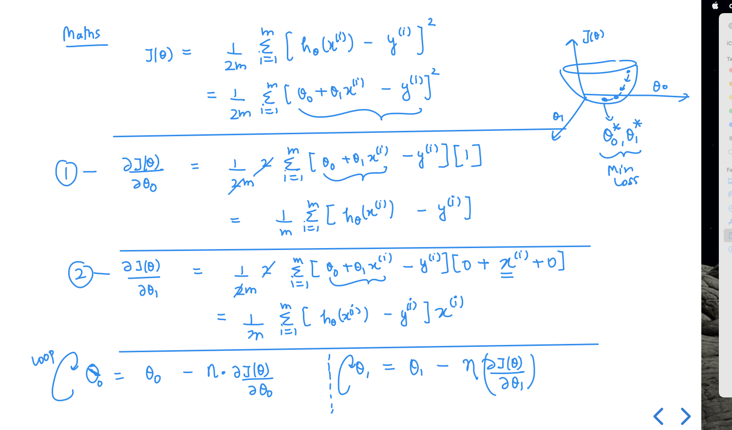
Decide Loss/Error Function
Given a training set, how do we learn, the best values for the parameters θ, so we define an error function that measures for each value of θ how close the predictions are to the actual y values.
The loss function is a measure of how close we are to the true/target value or in general, it is a measure of how good the algorithm is doing. The lower the loss the better.
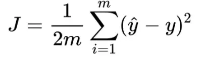
Hence, the loss function is mean squared error
Step 3
Training - an algorithm that reduces error on training data
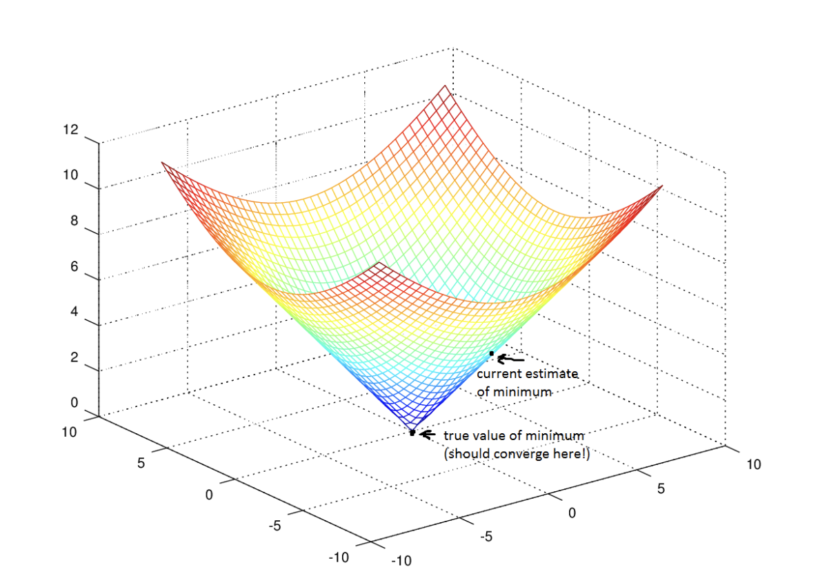
Starting with a random θ, we need an algorithm that iteratively improves θ by reducing J(θ) in each step and converges eventually to minimum error.
Find the parameters that minimize loss, i.e. make our model as accurate as possible.
Gradient Descent Algorithm

Gradient Descent
Imagine yourself walking through a valley with a blindfold on. Your goal is to find the bottom of the valley. How would you do it?
Gradient Descent Algorithm
(for linear regression)
LMS (Least Mean Squares) Update Rule
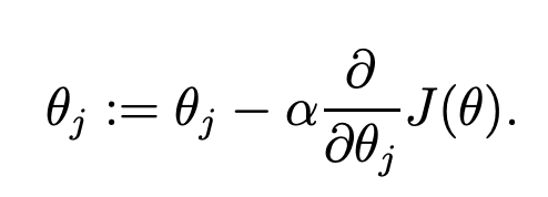
parameter = parameter-LR*(partial derivative of Loss w.r.t parameter)
Next, you find the partial derivatives of the loss function with respect to each theta parameter.
A partial derivative indicates how much total loss is increased or decreased if you increase theta parameter by a very small amount.
Training Loop
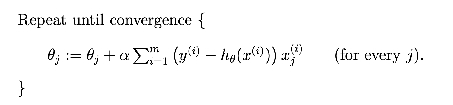
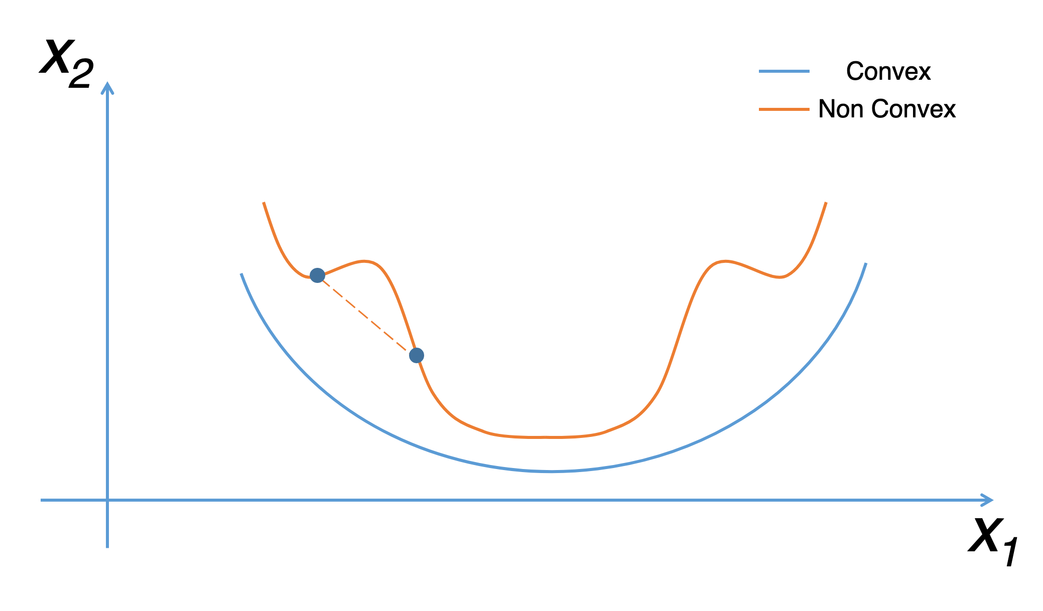
The optimisation problem we have posed here for linear regression has only one global, and no other local, optima; thus gradient descent always converges (assuming the learning rate α is not too large) to the global minimum. Indeed, J is a convex quadratic function.
Importance of Normalisation
Why do we need input features to be scaled or normalised ?

- The presence of feature value X in the formula will affect the step size of the gradient descent.
- The difference in ranges of features will cause different step sizes for each feature. For example - features like age, salary will have very different scales.
- To ensure that the gradient descent moves smoothly towards the minima and that the steps for gradient descent are updated at the same rate for all the features, we scale the data before feeding it to the model.
So we use, a acaling technique where the values are centered around the mean with a unit standard deviation.
This means that the mean of the attribute becomes zero and the resultant distribution has a unit standard deviation.
Here’s the formula for standardization:
is the mean of the feature values and is the standard deviation of the feature values.
R2 Score
Coefficient of determination is a statistical measure of how well the regression predictions approximate the real data points.
An R2 of 1 indicates that the regression predictions perfectly fit the data
Linear Regression
on dataset with multiple features

| Area (sqft) | Rooms | Locality Score | Price |
|---|---|---|---|
| 500 | 2 | 8 | 800k$ |
| 3200 | 8 | 7 | 16500$ |
| 900 | 4 | 10 | 12800$ |
| 1800 | 3 | 5 | .. |
Notation
-
n→number of features -
m→number of training examples -
X→input data matrix of shape (mxn) -
y→ target value (can be a Real number) -
x(i), y(i)→ith training example - x(i,j) →jth feature of ith training example
- theta → weights (parameters) of shape ((
n+1)x 1) -
y_hat→ hypothesis (outputs a real number)
| Area (sqft) | Rooms | Locality Score | Price |
|---|---|---|---|
| 500 | 2 | 8 | 800k$ |
| 3200 | 8 | 7 | 16500$ |
| 900 | 4 | 10 | 12800$ |
| 1800 | 3 | 5 | .. |
| ... | ... | ... | ... |
Step 1
Hypothesis function
Step 2
Loss function - mean squared error

Step 3
Training - learn the parameters by reducing the loss using gradient descent algorithm
Step 4
Prediction and Model Evaluation
Normal Equations
| Area (sqft) | Rooms | Locality Score | Price |
|---|---|---|---|
| 500 | 2 | 8 | 800k$ |
| 3200 | 8 | 7 | 16500$ |
| 900 | 4 | 10 | 12800$ |
| 1800 | 3 | 5 | .. |
Another approach to directly find the best parameters
Two approaches for error minimisation
-
Iterative Algorithm - Gradient Descent
-
Direct Way - Normal Equations/Closed Form Solution to directly get the optimal value of 'theta'
The Normal Equations
In this method, we will minimize J by explicitly taking its derivatives with respect to the θj ’s, and setting them to zero
So, you directly get the best theta, without iterating.

- For a simple problem like this, we can compute a closed form solution using calculus to find the optimal theta parameters that minimize our loss function
- But as a cost function grows in complexity, finding a closed form solution with calculus is no longer feasible. Hence an an iterative approach like gradient descent is required. It is more powerful which allows us to minimize a complex loss function.
Gradient Descent vs Closed Form Solution-I
- Closed form solution can be extremely expensive to compute, especially when X is large, the matrix 𝑋𝑇𝑋 can become huge and may not be practical to store it entirely in available RAM. A matrix of 10^5 x 10^5 will require a supercomputer!
- Even even the input matrix is large, the a slightly modified version of gradient descent algorithm allows to load a mini-batch of examples into memory, compute gradient and iteratively improve our model parameters.
Gradient Descent vs Closed Form Solution-II
- Binary Classification
- Logistic Regression
- Log Loss Error Function
- Gradient Descent
- Decision Boundary
- Implementation
Logistic Regression

Binary Classification
Is this email spam or not?
Is that borrower going to repay their loan?
Will those users click on the ad or not?
Is this fruit ripe or not?
Is it going to rain or not?
Logistic Regression
Classification algorithm based upon supervised learning.
The goal of the algorithm is to do binary classification, classify the input into one of the two classes.
The model outputs the probability of a categorical target variable Y belonging to a certain class.
Not just binary classification!
Logistic regression is often used for binary classification where there are two classes, but that classification can performed with any number of categories.

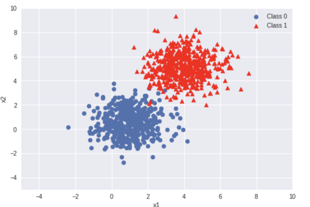
| x1 (Weight) | x2 (Sweetness) | Label |
|---|---|---|
| 8 | 7 | 🍎 1 |
| 10.1 | 9 | 🍎 1 |
| 12 | 11 | 🍎 1 |
| 8.5 | 3.8 | 🍎 1 |
| 3.5 | 5.0 | 🍊 0 |
| 2.7 | 2 | 🍊 0 |
| 6.4 | 4 | 🍊 0 |
| 9.7 | 8 | 🍎 1 |
| 4.4 | 3.2 | 🍊 0 |
Sample Training Data
Notations —
-
n→number of features -
m→number of training examples -
X→input data matrix of shape (mxn) -
y→true/ target value (can be 0 or 1 only) -
x(i), y(i)→ith training example -
θ → weights (parameters) of shape ((
n+1)x 1) -
y_hat(y with a cap/hat)→ hypothesis (outputs values between 0 and 1)
[x1 x2 x3 .... xn]
Input with
n features
(independent variables)
Model
(Hypothesis Fn)
y ∈ [0,1]
Probability value between 0 to 1
(We threshold later to decide the final label)
Step 1
Assume a Hypothesis function
Logistic regression is also a parametric method, which means it makes an assumption about the form of the function relating X and Y.
So we need to approximate y as a function of x.
Step 1
Assume a Hypothesis function
For a binary classification problem, we naturally want our hypothesis (y_hat) function to output values between 0 and 1 which means all Real numbers from 0 to 1.
So, we want to choose a function that squishes all its inputs between 0 and 1. One such function is the Sigmoid or Logistic function.
Sigmoid Function
Squashes the real values in the range between 0 and 1.

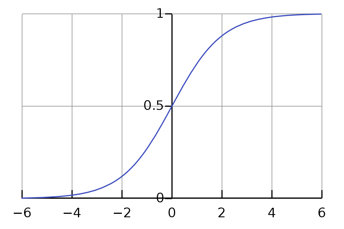
We can see that as z increases towards positive infinity the output gets closer to 1, and as z decreases towards negative infinity the output gets closer to 0.
Squashes the real values in the range between 0 and 1.
Logit Model
The logit model is a modification of linear regression that makes sure to output a probability between 0 and 1 by applying the sigmoid function.
Step 2
Loss Function - Binary Crossentropy
Step 3
Training - Learn model parameters using an algorithm like Gradient Descent.
Step 4 Predictions
Thresholding - Since the model predicts only probabilities, we need to put a certain threshold to decide the final label.
To predict the Y label—spam/not spam, cancer/not cancer, fraud/not fraud, etc.—we have to set a probability cutoff, or threshold, for a positive result. For example: “If our model thinks the probability of this email being spam is higher than 70%, label it spam. Otherwise, don’t.”
Implementation
Binary classification


Cat
Dog
Multi-class classfication


Deer
Egret
Langoor
Multi-label classfication

Classes:
Beeeater-Bird,
Honeybee
Binary Classification Models
Logistic Regression, Support Vector Machines, Perceptron etc were designed for binary classification only.
One approach for using binary classification algorithms for multi-classification problems is to split the multi-class classification dataset into multiple binary classification datasets and fit a binary classification model on each. Two different examples of this approach are the One-vs-Rest and One-vs-One strategies.
- The One-vs-Rest strategy splits a multi-class classification into one binary classification problem per class
- It involves splitting the multi-class dataset into multiple binary classification problems.
- A binary classifier is then trained on each binary classification problem and predictions are made using the model that is the most confident.
One Vs Rest Strategy (OvR)
- The one-vs-one approach splits the dataset into one dataset for each class versus every other class.
- We learn a model for every pair of classes, hence there are NC2 classifiers are learned for N classes.
- Each binary classification model may predict one class label and the label with the most predictions or votes is predicted by the one-vs-one strategy
- This approach is suggested for support vector machines (SVM) and related kernel-based algorithms
One Vs One Strategy (OvO)
scikit-learn library implements the OvR strategy by default when using these algorithms for multi-class classification.
- Linear Regression
- Logistic Regression
- Neural Networks
Parametric Models

Parametric models are those where the hypothesis function ℎ can be indexed by a fixed number of parameters. That is, the number of parameters of the model (hypothesis) are fixed and do not change with the increase in the data set size.
Non-Parametric Methods

The number of parameters describing the model/hypothesis usually grows with the dataset size. In decision trees, the parameters of the model, which is the tree size, is certainly not fixed and usually changes with the size of the data. For example, smaller datasets could be modeled with small size trees and larger datasets could require bigger trees.
Non-Parametric Methods
- KNN
- Classification & Regression
- Decision Trees
- Classification & Regression
These models are more flexible to the shape of the training data, but this sometimes comes at the cost of interpretability.
- KNN Idea
- Idea
- Implementation
- KNN for Regression & Classification
- Project
K-Nearest Neighbours

Steps
1) Load the training data.
2) Find out the similarity of test example with all points in the training data.
3) Sort the results according to distance / similarity score.
4) Take mean of nearest K values for regression, or take majority label from nearest K values for classification.
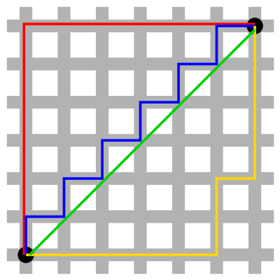
Distance Metric for Similarity
Euclidean Distance
Manhattan Distance
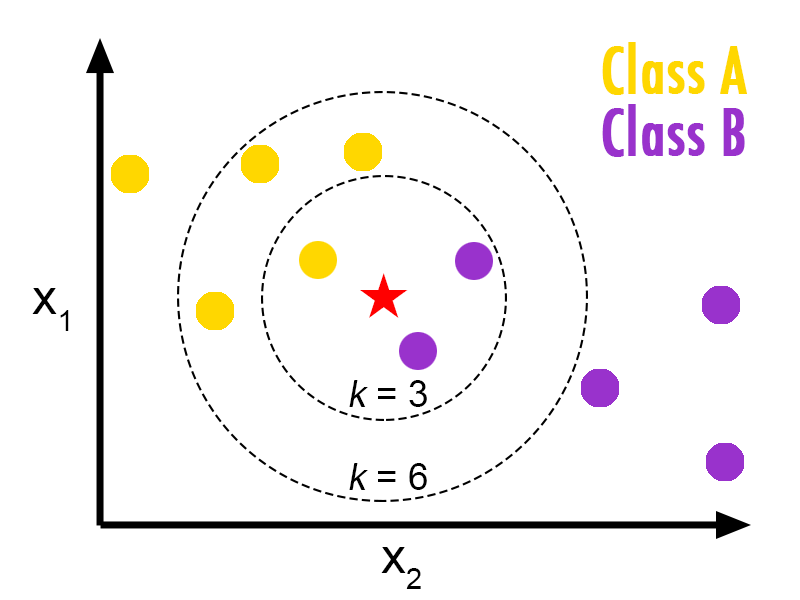
Choosing the right value of K.
KNN requires scaling of data because KNN uses the Euclidean distance between two data points to find nearest neighbors. Euclidean distance is sensitive to magnitudes
The features with high magnitudes will weight more than features with low magnitudes.
Advantages
k-NN doesn’t require a pre-defined parametric function f(X) relating Y to X makes it well-suited for situations where the relationship is complex/non-linear to be expressed with a simple linear model.Hence, KNN can be useful in case of nonlinear data.
There is no need to train a model for generalisation, that is why KNN is known as the simple and instance-based learning algorithm
The model can be used for both classification and regression tasks and can act as good baseline model.
Disadvantages
Since the model isn't learning anything, you have to iterate over entire dataset for making every prediction. This makes testing phase KNN slow on larger datasets.
Costlier in terms of time and memory, requires storing entire dataset for memory durin the prediction phase.

Project

Face
Recognition
- Unsupervised Learning
- Idea
- Clustering
- Dimensionality Reduction
- Applications
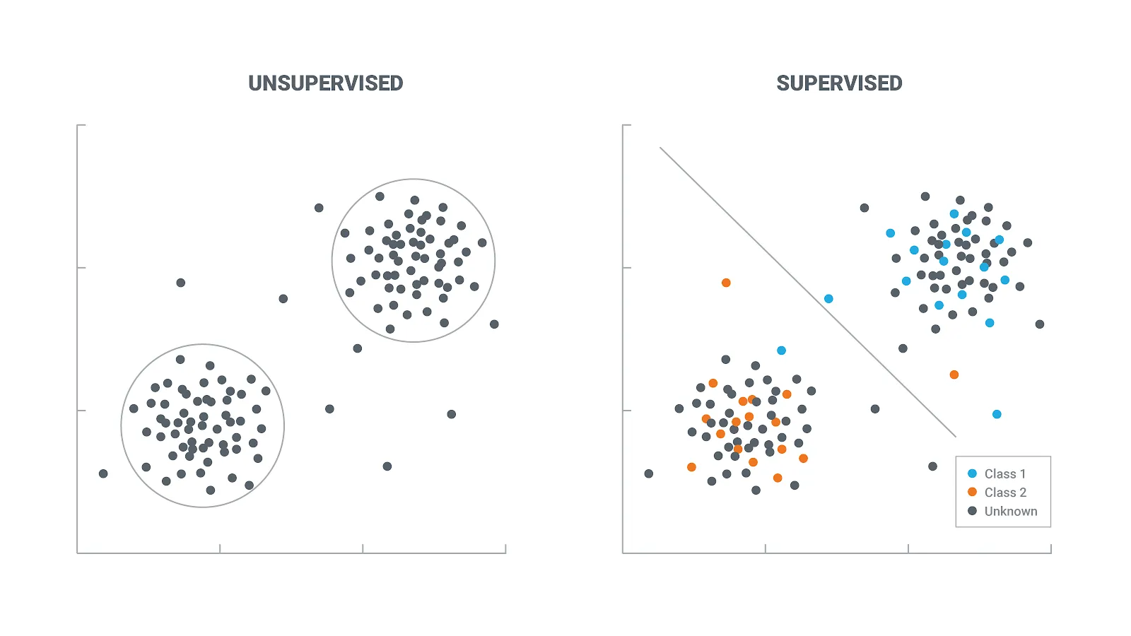
Unsupervised Learning

Unsupervised Learning
The goal of unsupervised learning to find underlying data structure of the dataset, or how to we group the data most usefully starting with a unlabelled dataset.
The two unsupervised learning techniques we will explore are clustering the data into groups by similarity and reducing dimensionality to compress the data while maintaining its structure and usefulness.
These tasks are helpful in doing Exploratory data analysis, customer segmentation, grouping similar images etc.
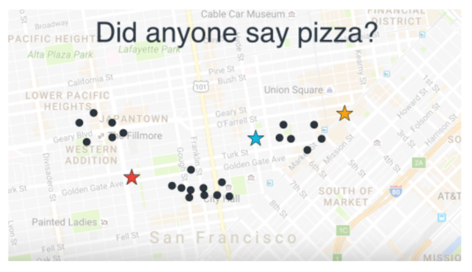
Clustering
The goal of clustering is to create groups of data points such that points in different clusters are dissimilar while points within a cluster are similar.
Techniques
K-Means Clustering,
Hierarchical Clustering
Dimensionality Reduction
This is about trying to reduce the complexity of the data while keeping as much of the relevant structure as possible. If you take a simple 128 x 128 x 3 pixels image (length x width x RGB value), that’s 49,152 dimensions of data.
If you’re able to reduce the dimensionality of the space in which these images live without destroying too much of the meaningful content in the images, then you’ve done a good job at dimensionality reduction.
Techniques
Principal Component Analysis,
Singular value decomposition,
T-SNE,
Deep Learning Techinques - Autoencoder
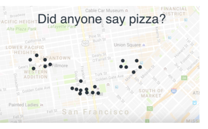
- Google Photos wants to cluster similar looking faces under one person category.
- Clustering news articles related to one topic under one heading.
- An advertising platform segments the population into smaller groups with similar purchasing habits so that advertisers can reach their target market.
- We often need reducing number of dimensions in a large data set to simplify models.
- Clustering Idea
- K-Means
- Implementation
- Project - Dominant Color Extraction
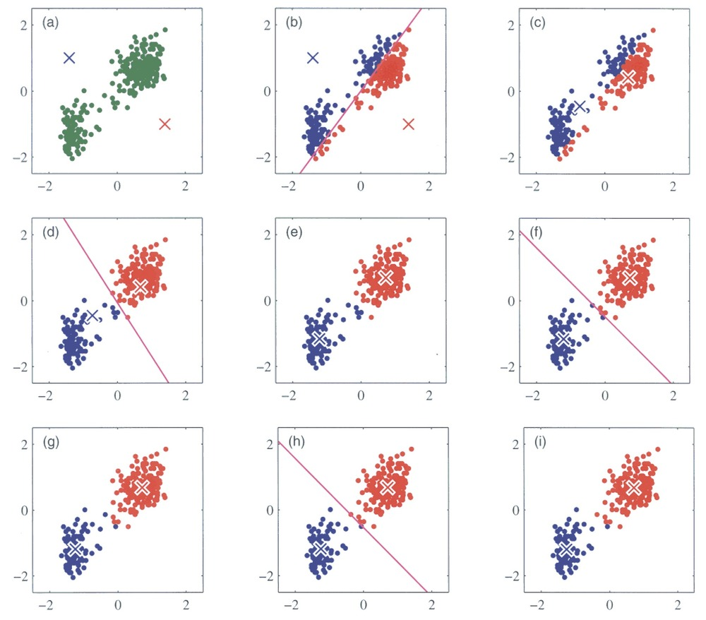
K-Means

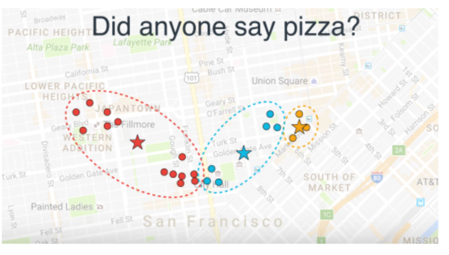
K-Means Clustering
The goal of clustering is to create groups of data points such that points in different clusters are dissimilar while points within a cluster are similar.
With k-means clustering, we want to cluster our data points into k groups.
The output of the algorithm would be a set of “labels” assigning each data point to one of the k groups.
In k-means clustering, the way these groups are defined is by creating a centroid for each group. The centroids are like the heart of the cluster, they “capture” the points closest to them and add them to the cluster.
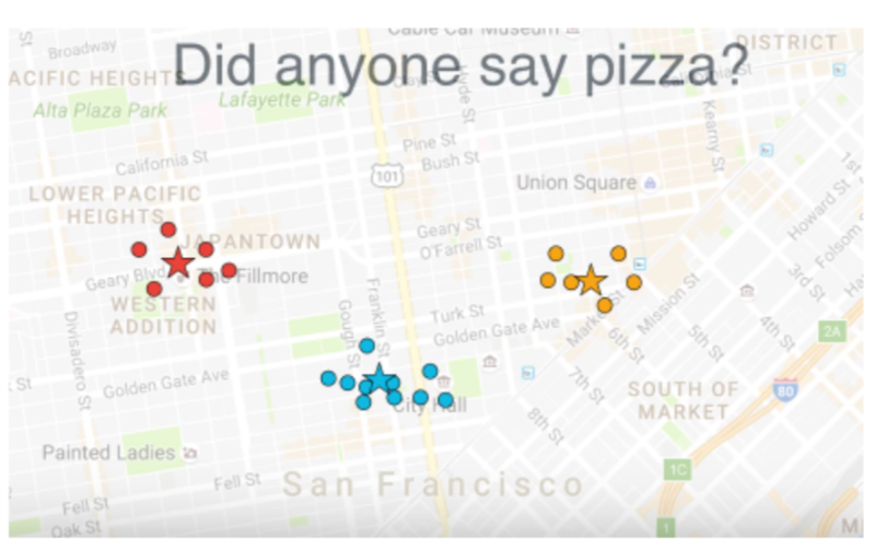
Steps
1) Define the k centroids - Initialise these at random
2a) Update cluster assignments. Assign each data point to one of the k clusters which is nearest.
2b) Update Centroids : Move the centroid to the center of their clusters.
Repeat Steps (2a, 2b) until convergence.Steps
Implemenation!
It works well on many realistic data sets, and is relatively fast, easy to implement, and easy to understand.


Things to Note
1) k-means is guaranteed to converge, the final cluster configuration to which it converges is not in general unique, and depends on the initial centroid locations.
2) It is actually possible for no data points to be assigned to a cluster in the Reassign Points step.
Further Reading . . .
1) Initialisation Strategies
2) Improvements :
K-Medians, K-Means++, EM Algorithm
2) Hierarchical Clustering
3) DBSCAN Algorithm