Becoming a Bayesian with Stan
Jim Savage
qplum Data-Science / FinTech Talks, Oct 21 2016
Why become a Bayesian?
- Decisions are made under uncertainty, which we want to deal with coherently. Uncertainty in model parameters. Uncertainty in the data given the parameters. Uncertainty in the model.
- Our data do not contain all the relevant information for the model. Especially in finance, we want to include information from outside our dataset.
- There are many non-deterministic things we are interested in. We want to model these jointly.
- Correspondingly, we want to be able to ask many questions to our models.
Why become a Bayesian?
You can learn from hierarchy
- Most data available have hierarchical structure (customers in postcode in state, firms in sub-sector in sector etc.)
- Most machine learning methods assume data are conditionally iid
- But we see in hierarchical datasets that similar observations are not conditionally iid.
- Using simpler models that take into account within-group covariance can result in far better predictions than complex machine learning methods.
- Also helps us think through causal structure, by controlling for unobserved information fixed at the group level.
Why become a Bayesian? An example
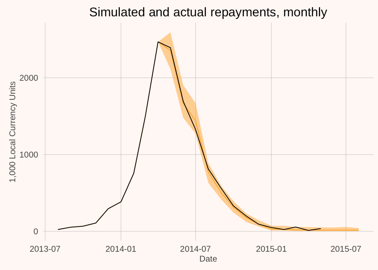
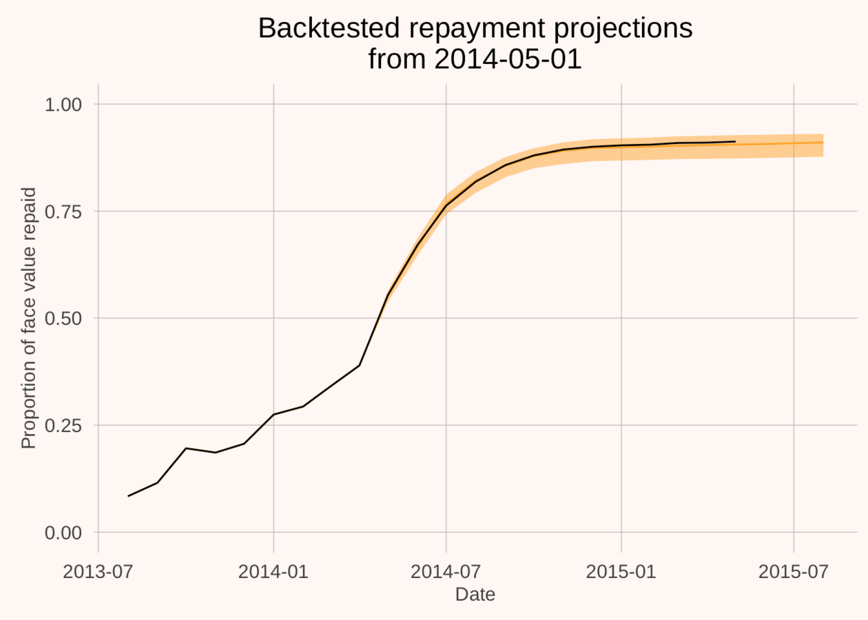
- Train model on 150 loans in Sub-Saharan Africa
- (Out of sample) predicted the repayments of 2000 different rural microfinance loans
- Cumulative error = less than 1 per cent.
Why become a Bayesian? An example


Why become a Bayesian? An example
Why become a Bayesian? An example
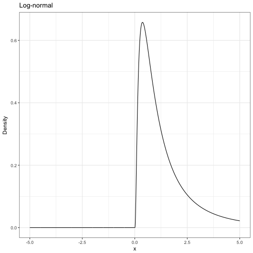
We get to build models that put weight on plausible values, and none on impossible values.

How to become a Bayesian
- Flip your thinking from pattern-discovery to pattern generation (thinking through generative structure)
- Learn Modern Statistical Workflow (this lecture!)
- Install Stan and implement a couple of the models in the manual
- Join Stan Users groups.google.com/forum/#!forum/stan-users
Modern Statistical Workflow: why?
- As the amount of data that we're able to process grows, we can estimate more complex models.
- More complex models can give us better insights,
- But also be far more likely to break.
- Need a workflow that helps us develop high quality models that don't break.
Modern Statistical Workflow: the punchline
- Plot data, think through generative process. Discuss it with critical friends
- Write out the probability model (priors and likelihood)
- Simulate from the model with known parameters
- Estimate your model to make sure you can recapture the parameters
- Estimate the model on real data
- Check the model fit to make sure it estimated properly. (You will be amazed at how many of the models that you are using today haven't!)
- (If you have more than one model) model comparison
- Inference
- Iterate, building richer specifications
Outline
- Modern Statistical Workflow (done!)
- A very gentle introduction to generative models
- A finance demonstration: finite mixture model with time-varying mixture probabilities
Generative models: what are they?
Technical
A joint distribution of all the unknowns in the model. Unknowns = outcomes, parameters, latent variables.
Street
A model in which we deal coherently with both uncertainty in the dependent variables and all the parameters of the model.
Generative models: Why not?
“Bayesian inference is hard in the sense that thinking is hard” - Don Berry
- No black box solutions
- Actually have to know the model that you are estimating
- A lot is not automated.
- Historically quite difficult.
But now we just use Stan.
Generative models: human heights
Let's say we want a model of human heights using only sex to predict. I want to build a model that can help answer several questions:
- If I know that someone is female, what do I predict their height to be on average?
- If I don't know what sex someone is, what do I predict their height to be?
- How uncertain am I about the average height of men?
- How tall do I expect a man at the 90th percentile of height to be?
Generative models: Parts of the model
- Explanatory variable: sex (also known as feature, covariance, auxiliary variable, etc.). Explanatory variables are known with certainty, both in and out of sample.
- Outcome: height (also known as response, dependent variable, etc.). Given the explanatory variable, many possible values of outcome are possible. We treat it as a random variable.
Generative models: Parts of the model
- Distribution. We need to make (informed) assumptions about how the outcome is distributed given the explanatory variables. For this purpose, let's let
\( \mbox{female height} \sim \mbox{normal}(\mbox{average}_{f}, \sigma) \) and
\( \mbox{male height} \sim \mbox{normal}(\mbox{average}_{m}, \sigma) \) (same standard deviation)
- Parameters Values that map our explanatory variables to our outcome via the distribution(s). In this case, the mean height of men, the mean height of women, the standard deviation of people, and the sex shares will be sufficient.
Generative models: drawing inference from model output
- Let's simulate this model with known parameters.
library(dplyr)
# Random draws of height for 10k people from normal distribution
# 51% female
heights_women <- rnorm(n = 5100, mean = 165, sd = 8)
# 49% male
heights_men <- rnorm(n = 4900, mean = 175, sd = 8)
# Organize the data into a data.frame
heights_people <- data_frame(Sex = c(rep("f", 5100), rep("m", 4900)),
                             height = c(heights_women, heights_men))
- This is called Monte Carlo sampling. Given enough draws from a distribution, we can calculate any statistic to an arbitrary degree of accuracy.
Generative models: drawing inference from model output
# Female height on average
heights_people %>%
  filter(Sex=="f") %>%
  summarize(mean(height))
# A tibble: 1 × 1
  `mean(height)`
           <dbl>
1       165.0282
# Human height on average
heights_people %>%
  summarize(mean(height))
# A tibble: 1 × 1
  `mean(height)`
           <dbl>
1       169.9139
Generative models: drawing inference from model output
# Standard deviation of height of men
heights_people %>%
  filter(Sex=="m") %>%
  summarize(sd(height))
# A tibble: 1 × 1
  `sd(height)`
         <dbl>
1     7.986179
# Height of males at the 90th percentile
heights_people %>%
  filter(Sex=="m") %>%
  summarize(quantile(height, 0.9))
# A tibble: 1 × 1
  `quantile(height, 0.9)`
                    <dbl>
1                185.1751
Generative models: What is wrong with this model?
Do you believe this model?
Generative models: What is wrong with this model?
- No uncertainty in parameters
- Have not used any data!
- The the distributional assumptions valid?
We want to spend some time working through these problems.
Some statistical background: random variables
A variable is a random variable if its value is not controlled/deterministic. It is subject to chance.
We think about the following as random variables:
- Outcomes
- Parameters
- Latent Variables
Some statistical background: Probability density functions
A probability density function tells us the relative probability of observing certain values of a random variable.
- We denote the density of random variable \( X \) with \( p(X) \)
- \( p() \) is overloaded, meaning \( p(X) \) could have a different form to \( p(Y) \)
- The area under the curve \( p(X) \) is 1
Some statistical background: Probability density functions


Some statistical background: Joint densities
Some statistical background: Joint densities
Some statistical background: Marginal distributions
Some statistical background: Conditional distribution
Some statistical background: Density
Some statistical background: Likelihood
- For a given density function with fixed parameters, and a fixed observation of the outcomes \( Y \), Likelihood is the product of each data point's density.
- Because densities are typically small, taking logs of densities and summing is prefered in many cases. In this case we have the Log Likelihood.
Some statistical background: Likelihood
Generative models: Introducing uncertainty to our model
Our model has several random variables:
- The average heights of men and women
- The standard deviation of heights (assume same for all people)
- The distribution of sexes.
- The outcome: The distribution of heights given gender and parameters.
A more complete generative model is the joint density of these
\[ p(\mbox{Heights}, \mbox{average}_{m}, \mbox{average}_{f},\sigma,\mbox{distribution of sexes}) \]
Generative models: Introducing uncertainty to our model
This factors into conditional densities \[ p(\mbox{Heights}, \mbox{average}_{m}, \mbox{average}_{f},\sigma, \mbox{distribution of sexes}) \]
\[ = p(\mbox{Heights}|\, \mbox{average}_{m}, \mbox{average}_{f},\sigma, \mbox{distribution of sexes})\times \] \[ p(\mbox{average}_{m}|\, \mbox{average}_{f}, \sigma,\mbox{distribution of sexes})\times \] \[ p(\mbox{average}_{f}|\, \sigma,\mbox{distribution of sexes})\times \] \[ p(\sigma|\,\mbox{distribution of sexes})\times \] \[ p(\mbox{distribution of sexes}) \]
And if these are independent \[ = p(\mbox{Hghts}|\mbox{params})\times p(\mbox{av}_{m})\times p(\mbox{av}_{f})\times p(\sigma)\times p(\mbox{sex distr.}) \]
Generative models: Incorporating uncertainty
- Before, we simulated from \( p(\mbox{Heights}|\mbox{params}) \) taking params to be known
- Now we want to generate draws from the joint density on the previous slide.
The process is simple:
- Specify distributions that make sense to you given your expertise for \( p(\mbox{av}_{m}, \mbox{av}_{f}, \sigma, \mbox{sex distr.}) \)
- Assuming independence \( p(\mbox{av}_{m}) \), \( p(\mbox{av}_{f}) \), \( p(\sigma) \), and \( p(\mbox{sex distr.}) \).
Generative models: Incorporating uncertainty
Then
- Draw \( \mbox{params} \) from these distributions
- Parameterize the data distribution with these draws
- Draw \( \mbox{Heights} \) from the newly parameterized \( p(\mbox{Hghts}|\mbox{params}) \)
Generative models: Still haven't used any data!
- Note that we are currently using \( p(\mbox{av}_{m}, \mbox{av}_{f}, \sigma, \mbox{sex distr.}) \) without having seen any data.
- Want to condition our parameter estimates on some observed data: observed heights and observed sexes. That is, we want \( p(\mbox{av}_{m}, \mbox{av}_{f}, \sigma, \mbox{sex distr.}|\, \mbox{observed heights, sexes}) \)
Generative models: Bayes rule
Let's call our collection of parameters \( \theta \) and our observed heights \( y \). Bayes rule tells us that
\[ p(\theta|\, y) = \frac{p(y|\, \theta)\, p(\theta)}{p(y)} \]
Since \( p(y) \) does not depend on \( \theta \), we can re-write this in proportional form
\[ p(\theta|y)\propto p(y|\, \theta)\, p(\theta) \]
Generative models: All we need to do is specify priors and likelihood
\[ p(\theta|\, y)\propto p(y|\, \theta)\, p(\theta) \]
- We have \( p(\theta) \)—this is what we were using to parameterize the model before. This is called the prior
- We have \( p(y|\, \theta) \)—this is the assumed distribution given the parameters. This is the data model for unknown \( y \), or the Likelihood for fixed \( y \).
- We can use this to estimate our “updated” distribution for the parameters: \( p(\theta|\, y) \). This is the posterior
Generative models: All we need to do is specify priors and likelihood
- If you can form priors for your parameters and come up with a conditional density for your data, Stan will help you estimate the posterior.
- We can use priors to help us incorporate information not in the data.
A real toy model
- Sometimes stocks behave as thought prices move according to a random walk
- Other times they look as though there is momentum
How do we know which is which? Can we form an understanding of this?
A real toy model
Let's say there are two possible models that describe daily returns:
Model 1: a random walk model \[ r_{t} \sim \mbox{normal}(\alpha_{1}, \sigma_{1}) \]
Model 2: simple AR(1) momentum \[ r_{t} \sim \mbox{normal}(\alpha_{2} + \rho_{1} r_{t-1}, \sigma_{2}) \]
A real toy model
Which model? \[ p(\mbox{Model 1} | \mu) = \mbox{Logit}^{-1}(\mu_{t}) \]
and
\[ \mu_{t} \sim \mbox{normal}(\alpha_{3} + \rho_{2} \mu_{t-1} + f(\mathcal{I}_{t}), \sigma_{3}) \]
Where \( f(\mathcal{I}_{t}) \) is a function of information available at the beginning of day \( t \). For this exercise, we assume
\[ f(\mathcal{I}_{t}) = \beta r_{t-1} \]
Simulate some data with known parameters
(See R session)
Simulate some data with known parameters (if you want to play at home)
library(rstan); library(ggplot2); library(dplyr); library(reshape2)
options(mc.cores = parallel::detectCores())

# Set some fake parameters
alpha1 <- -0.01; alpha2 <- 0.015
rho1 <- 0.95; rho2 <- 0.8
beta <- 0.5

sigma1 <- 0.05; sigma2 <- 0.03; sigma3 <- 0.3
T <- 500
r <- rep(NA, T)
r[1] <- 0

mu <- rep(NA, T)
z <- rep(NA, T)
mu[1] <- 0
z[1] <- 1
Simulate some data with known parameters
# Simulate the data series
for(t in 2:T) {
  mu[t]  <- rho1 * mu[t-1] + beta*(r[t-1]) + rnorm(1, 0, sigma3)
  prob <- arm::invlogit(mu[t])
  if(z[t]==1) {
    # random walk state
    r[t] <- rnorm(1, alpha1, sigma1)
  } else {
    # momentum state
    r[t] <- rnorm(1, alpha2 + rho2*r[t-1], sigma2)
  }
}

plot.ts(r)
plot.ts(arm::invlogit(mu))
Check to see that known "unknowns" can be re-captured
(See R session)
Quick outline of a Stan model
-
data: declare the data you will give the model -
transformed data: make any changes to the data -
parameters: declare the unknowns -
transformed parameters: sometimes the parameters we want are a function of pars. that are easy to estimate -
model: declare the priors and likelihood
Syntax is somewhere between R and C++:
- R-like loops, very similar indexing
- C++-like static typing, commenting, finish lines with ;
Log sum exp
Before writing the model: note that if we see a datapoint \( r_{t} \), it has the likelihood (for parameter vector \( \theta \)):
\[ p(r_{t}| \theta) = \mbox{Logit}^{-1}(\mu_{t})\mbox{normal}(r_{t} |\, \alpha_{1}, \sigma_{1}) +\\ (1-\mbox{Logit}^{-1}(\mu_{t}))\mbox{normal}(r_{t} |\, \alpha_{2} + \rho r_{t-1}, \sigma_{1}) \]
Because we work in logs, we want \( \log(p(r_{t}| \theta)) \). For this we use the log_sum_exp functon, defined as: log_sum_exp(a, b) = log(exp(a) + exp(b)).
Our Stan model
// saved as switching_model.stan
data {
  int T;
  vector[T] r;
}
parameters {
  vector[T] mu;
  vector[2] rho;
  real beta;
  vector<lower = 0>[3] sigma;
  vector[3] alpha;
}
model {
  // priors
  mu[1:2] ~ normal(0, .1);
  sigma[1:2] ~ cauchy(0, 0.05);
  sigma[3] ~ cauchy(0, 0.5);
  rho ~ normal(1, .1);
  beta~ normal(.5, .25);
  alpha[1:2] ~ normal(0, 0.1);
  alpha[2] ~ normal(0, 1);

  // likelihood
  for(t in 3:T) {
    mu[t] ~ normal(alpha[3] + rho[1]*mu[t-1] + beta* r[t-1], sigma[3]);

    target += log_mix(inv_logit(mu[t]),
                      normal_lpdf(r[t] | alpha[1], sigma[1]),
                      normal_lpdf(r[t] | alpha[2] + rho[2] * r[t-1], sigma[2]));
  }
}
Estimating the model from R
library(rstan)
options(mc.cores = parallel::detectCores())
compiled_model <- stan_model("switching_model.stan")
posterior_draws <- sampling(compiled_model,
                            data = list(r = r,
                                        T = T))

print(fit, pars = c("alpha", "beta", "sigma"))
Checking model fit
install.packages("shinystan")
shinystan::launch_shinystan(posterior_draws)
Checking to see you reclaimed the data
outcome_data <- test_model %>%
  as.data.frame() %>%
  select(contains("mu")) %>%
  melt() %>%
  group_by(variable) %>%
  summarise(lower = quantile(value, 0.1),
            median = median(value),
            upper = quantile(value, 0.9)) %>%
  mutate(date = 1:n(),
         true_mu = mu)

outcome_data %>%
  ggplot(aes(x = date)) +
  geom_ribbon(aes(ymin = arm::invlogit(lower),
                  ymax = arm::invlogit(upper)),
              fill= "orange", alpha = 0.4) +
  geom_line(aes(y = arm::invlogit(median))) +
  geom_line(aes(y = arm::invlogit(true_mu)), colour = "red")
Taking the model to real data
(See R session)
Taking the model to real data
# Now with real data!
aapl <- Quandl::Quandl("YAHOO/AAPL")

aapl <- aapl %>%
  mutate(Date = as.Date(Date)) %>%
  arrange(Date) %>%
  mutate(l_ac = log(`Adjusted Close`),
         dl_ac = c(NA, diff(l_ac))) %>%
  filter(Date > "2015-01-01")

aapl_mod <- sampling(compiled_model, data= list(T = nrow(aapl), r = aapl$dl_ac*100))

print(aapl_mod, pars = c("alpha", "sigma", "rho", "beta"))
Taking the model to real data
plot1 <- aapl_mod %>%
  as.data.frame() %>%
  select(contains("mu")) %>%
  melt() %>%
  group_by(variable) %>%
  summarise(lower = quantile(value, 0.95),
            median = median(value),
            upper = quantile(value, 0.05)) %>%
  mutate(date = aapl$Date,
         ac = aapl$l_ac) %>%
  ggplot(aes(x = date)) +
  geom_ribbon(aes(ymin = arm::invlogit(lower), ymax = arm::invlogit(upper)), fill= "orange", alpha = 0.4) +
  geom_line(aes(y = arm::invlogit(median))) +
  lendable::theme_lendable() +
  xlab("Date") +
  ylab("Probability of random walk model")
Taking the model to real data
plot2 <- aapl_mod %>%
  as.data.frame() %>%
  select(contains("mu")) %>%
  melt() %>%
  group_by(variable) %>%
  summarise(lower = quantile(value, 0.95),
            median = median(value),
            upper = quantile(value, 0.05)) %>%
  mutate(date = aapl$Date,
         ac = aapl$`Adjusted Close`) %>%
  ggplot(aes(x = date, y = ac)) +
  geom_line() +
  lendable::theme_lendable() +
  xlab("Date") +
  ylab("Adjusted Close")

gridExtra::grid.arrange(plot1, plot2)