Statistical Comparison of Various Dayside Magnetopause Reconnection X-line Prediction Models

Ramiz A. Qudsi, Brian Walsh, J. Broll, Stein Haaland
Boston University, Los Alamos National Lab, Max-Planck Institute
*(qudsira@bu.edu)
1, * 1 2 3
1 2 3


Outline:
- Region of interest
- Location of x-line
- Different models
- Data
- Results
- Discussions
Qudsi (qudsira@bu.edu)
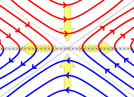
The BASICS
Qudsi (qudsira@bu.edu)
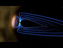
Source: NASA
Qudsi (qudsira@bu.edu)
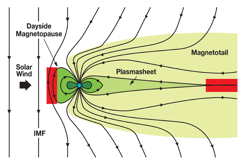
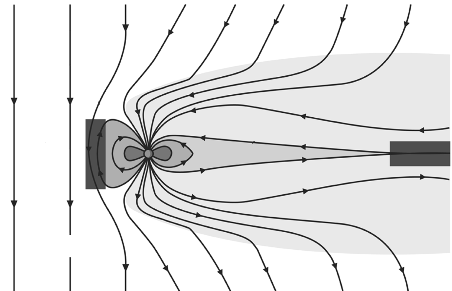
Region of interest:
Qudsi (qudsira@bu.edu)
[Broll et al., 2017]
Source: wikipedia
Qudsi (qudsira@bu.edu)
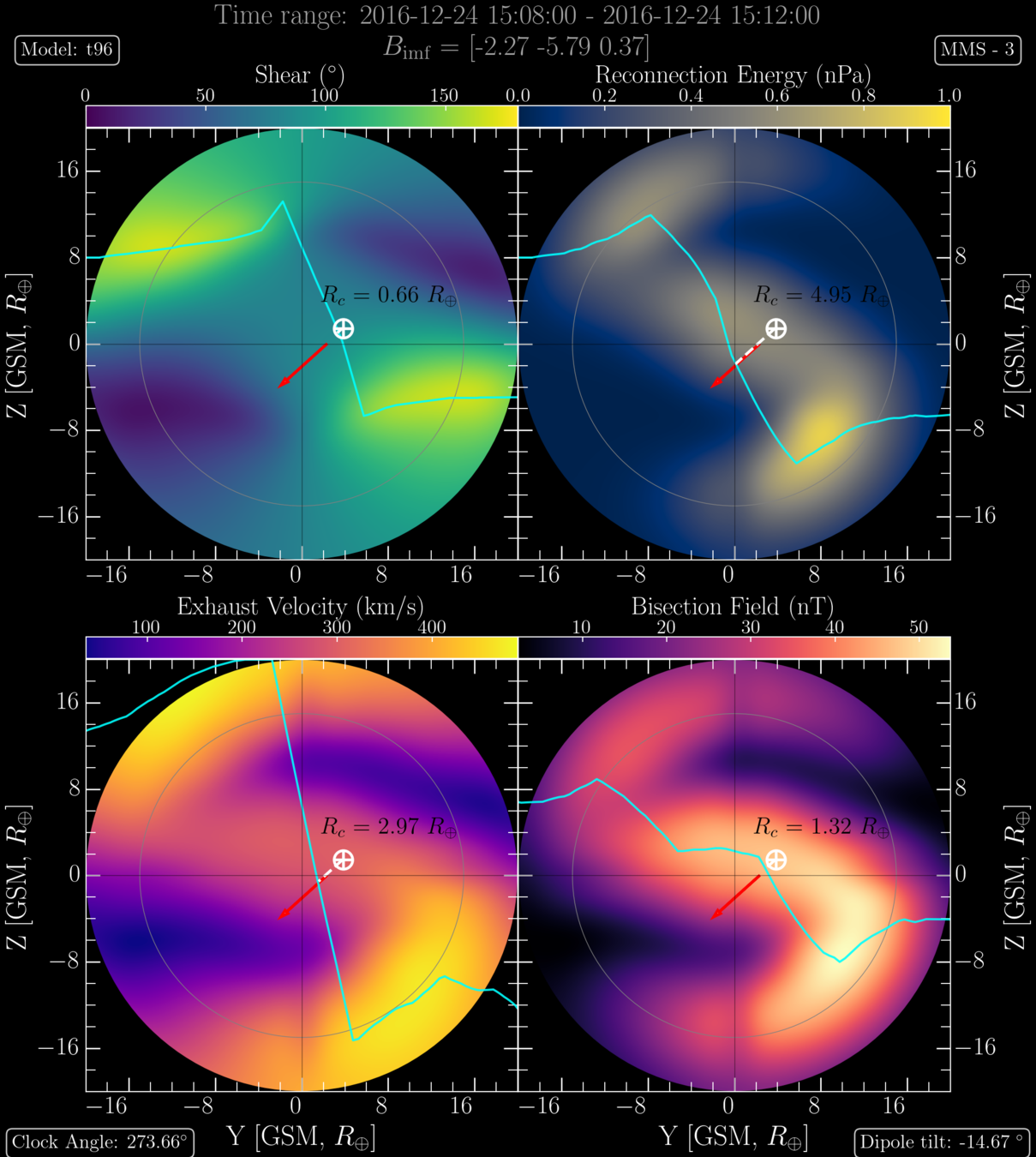
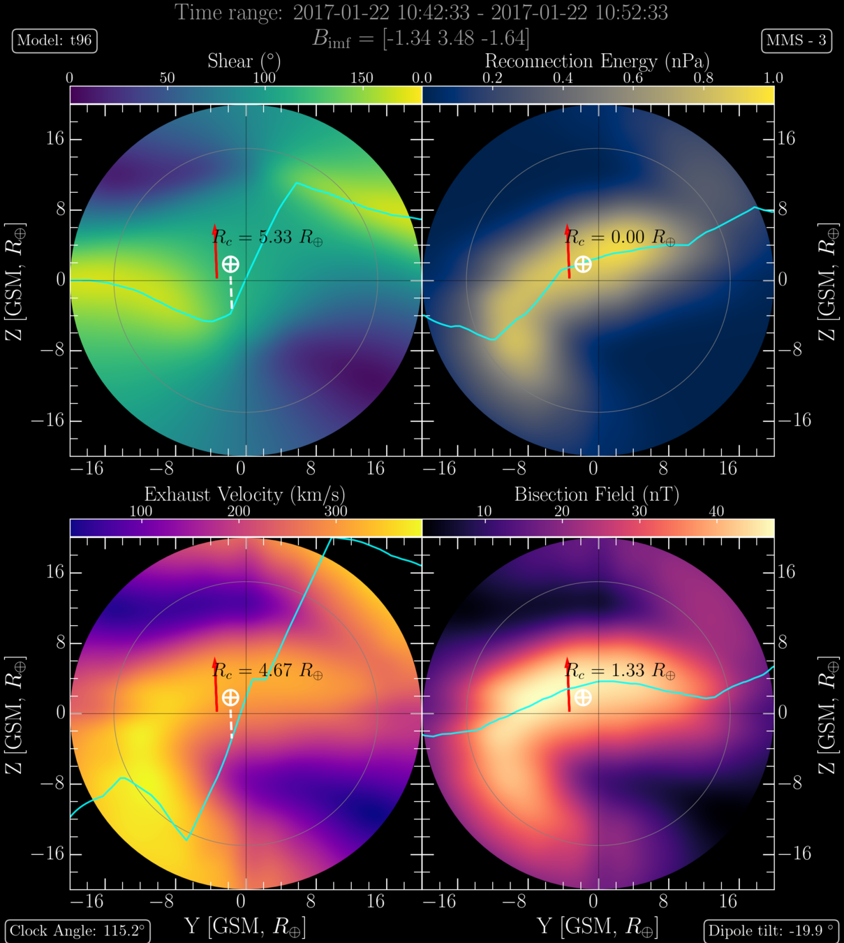
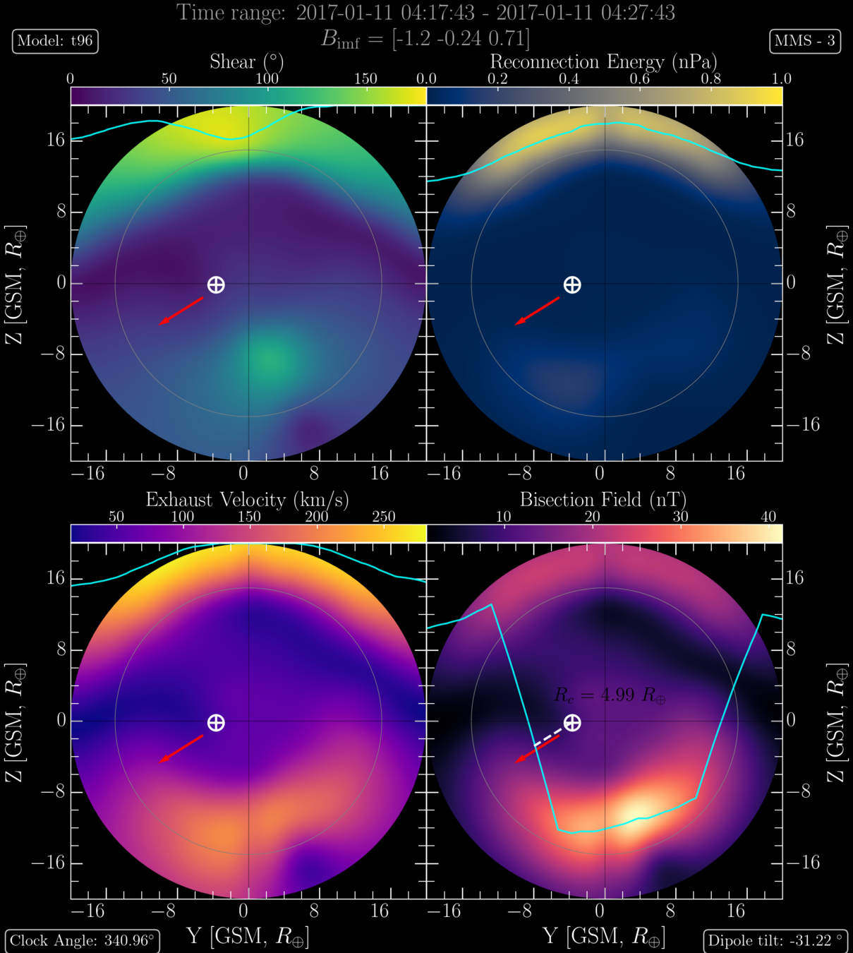
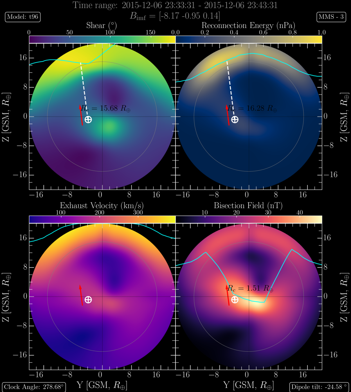
Location of x-line: Models
Local field bisection [Moore et al., 2002]
Maximum exhaust speed [Swisdak and Drake, 2007]
Maximum magnetic shear [Trattner et al., 2007]
Maximum reconnecting field energy [Hesse et al., 2013]
Qudsi (qudsira@bu.edu)
Magnetic shear [Trattner et al., 2007]:
Local field bisection [Moore et al., 2002]:
Reconnection field energy [Hesse et al., 2013]:
Exhaust speed [Swisdak and Drake, 2007]:
sh: magnetosheath
msp: magnetosphere
Location of x-line: Models
Qudsi (qudsira@bu.edu)
DATA
Qudsi (qudsira@bu.edu)
Data:
Solar
Wind
OMNI
Cooling-2001 Model
Magnetosheath
Magnetopause
Shue-1998 Model
T-96 and IGRF Model
Magnetospheric Fields
Qudsi (qudsira@bu.edu)
Data
Solar Wind data: OMNI (propagated to the magnetopause)
Magnetosheath data: MMS (FPI and FGM)
Magnetospheric magnetic field: Models (T96 or T05 and IGRF)
Magnetosheath magnetic field: Models (Cooling model)
x
z
y
GSM coordinate system
Qudsi Center for Space Physics, BU qudsira@bu.edu
Methodology
Qudsi (qudsira@bu.edu)
Methodology
- Look at the instances when MMS observed a jet reversal while crossing the magnetopause.
Qudsi (qudsira@bu.edu)
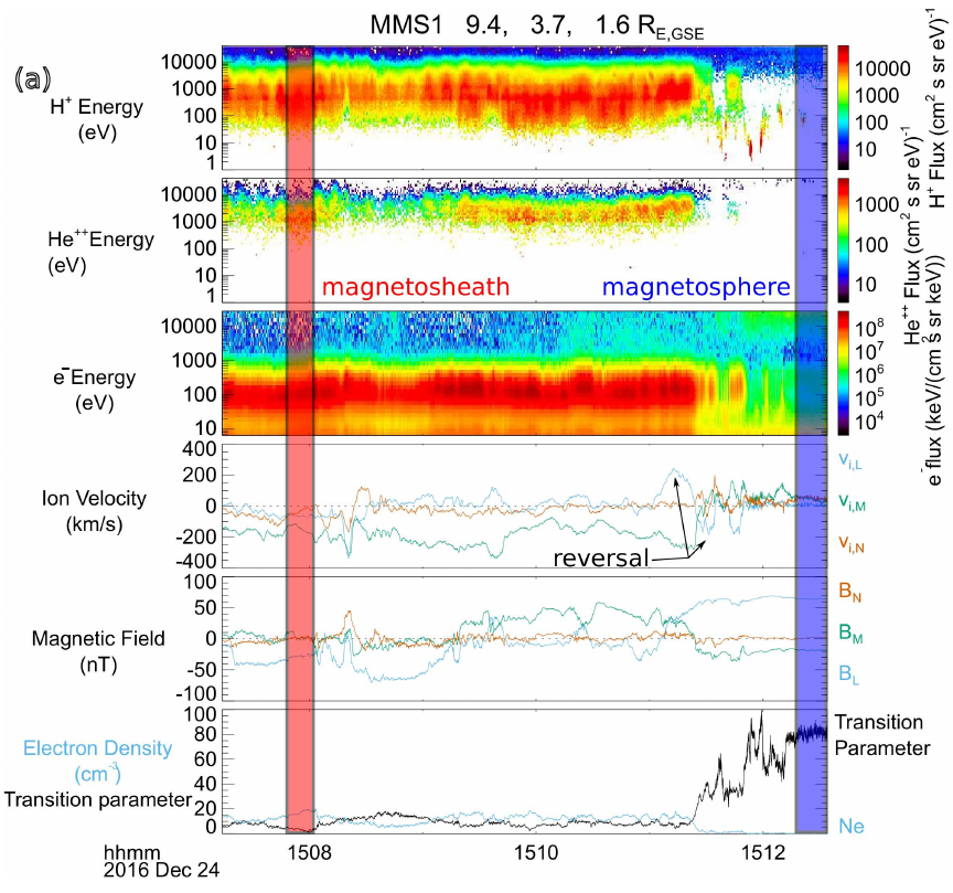
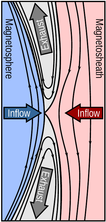
Magnetosheath
Magnetosphere
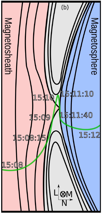
[Broll et al., 2017]
Qudsi (qudsira@bu.edu)
Methodology
- For the observed parameters of IMF, Magnetosheath and Magnetosphere and Magnetopause find the model predicted x-line locations.
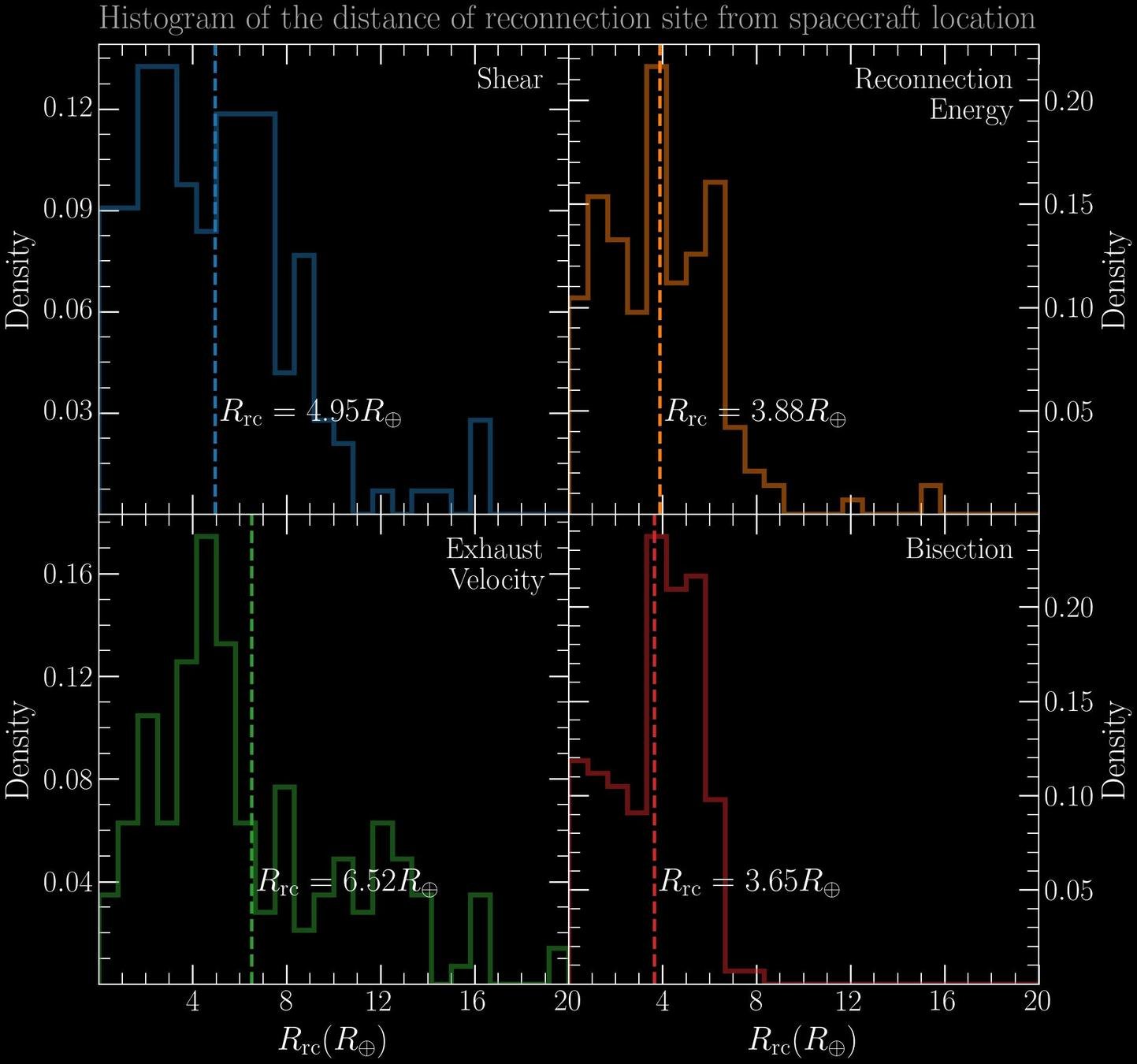
- Find the distance of x-line from MMS, along the magnetopause, for different models.
- Look at the statistical distribution of distances (histogram etc.) for different models.
Qudsi (qudsira@bu.edu)
- Look at the instances when MMS observed a jet reversal while crossing the magnetopause.
RESULTS
Qudsi (qudsira@bu.edu)
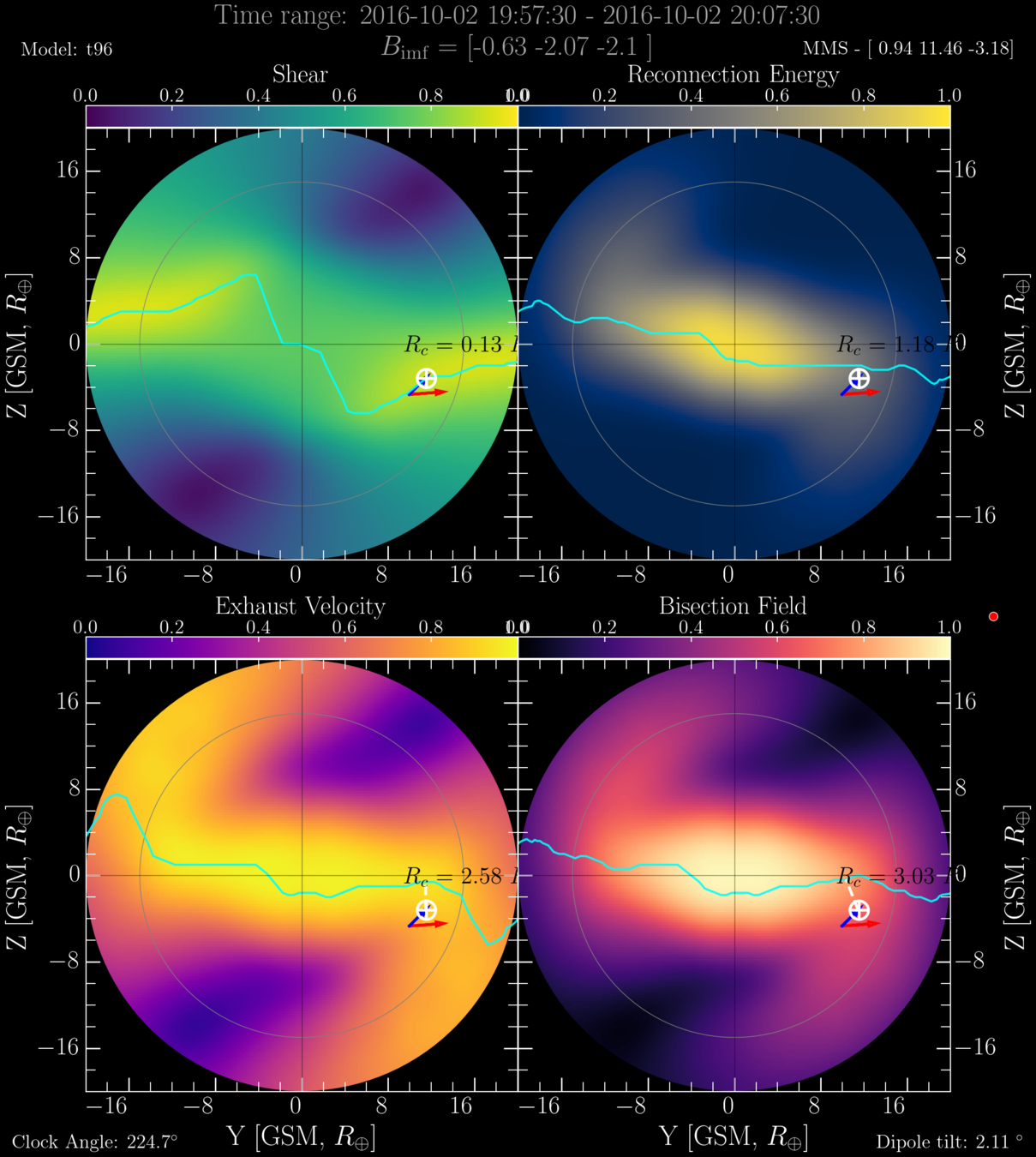
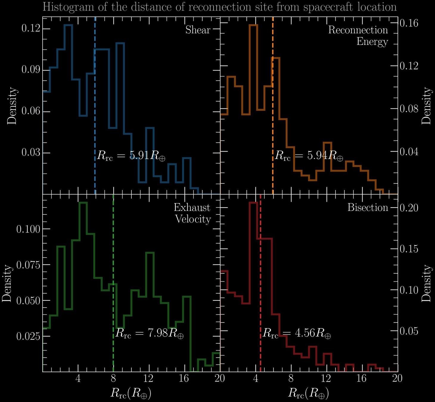
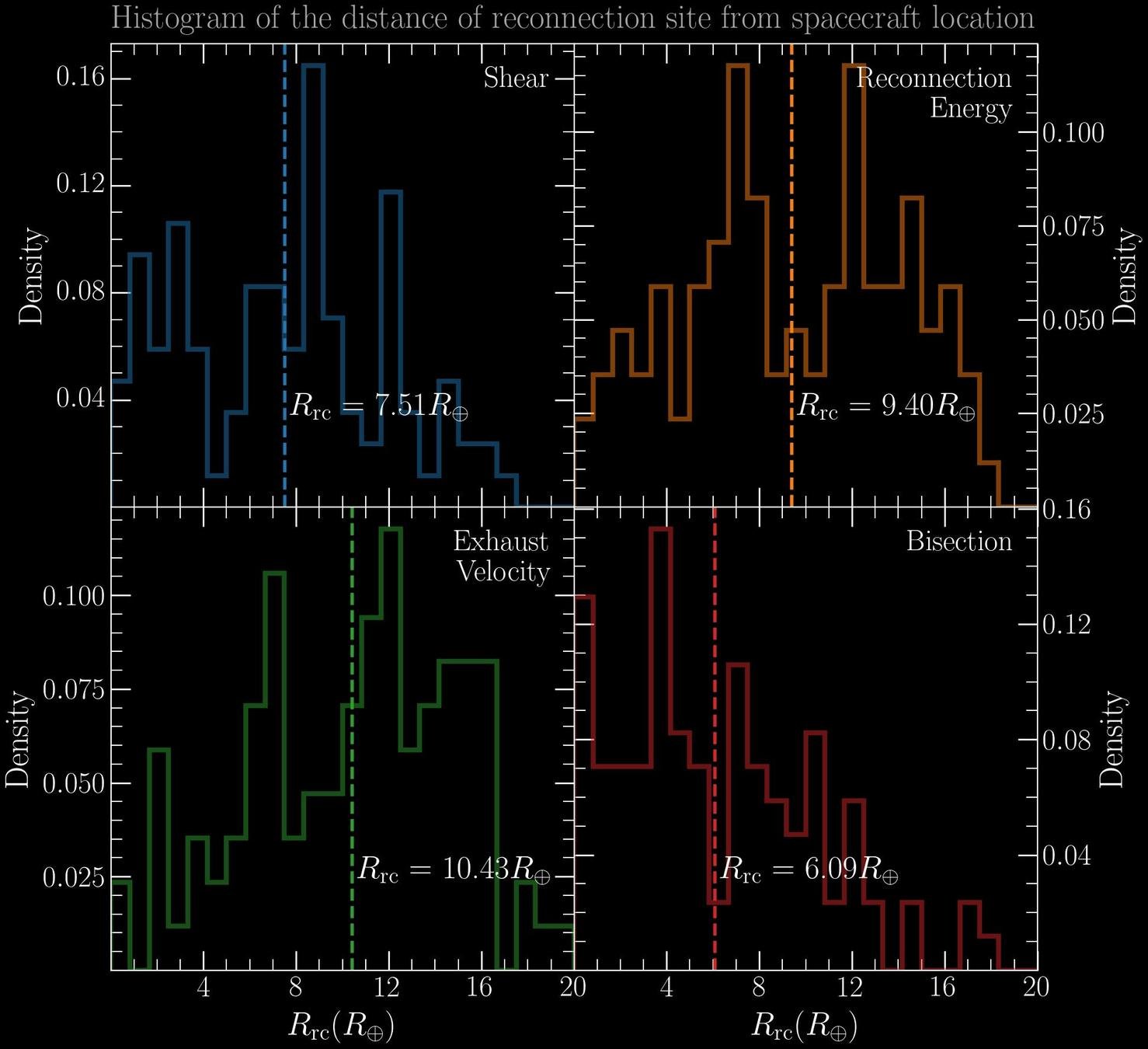
The maximum shear model:
The maximum exhaust velocity model
Qudsi (qudsira@bu.edu)

DISCUSSIONS
Qudsi (qudsira@bu.edu)
Discussions:
For negative z-component of IMF, reconnection energy and bisection field models both give very similar statistics.
For positive z-component, shear and bisection model seem to do the best job of predicting the expected x-line
Statistically, bisection field model seem to perform better than other models for different IMF and magnetopause conditions.
Qudsi (qudsira@bu.edu)
Thank You!
Link to the presentation
Qudsi (qudsira@bu.edu)