Qualifying Exam

Rebecca Barter

advised by

Jas Sekhon and Bin Yu

May 15, 2018

Projects I'm going to talk about

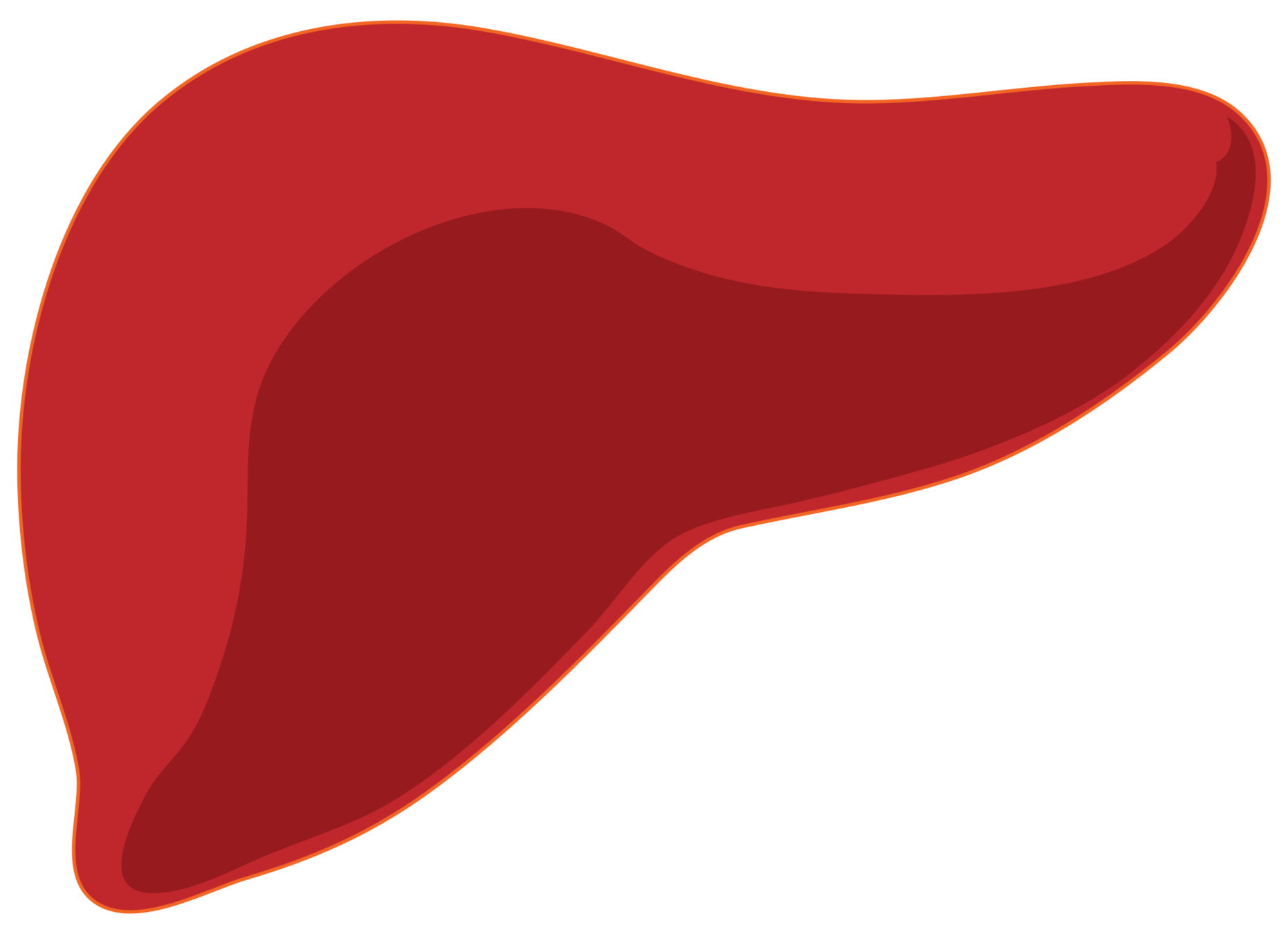
The fundamental problem of transplantation

Current approaches to increasing supply

Live donor chains

Blum et al. (2015, 2016): Finding the optimal chain using stochastic matching on a graph

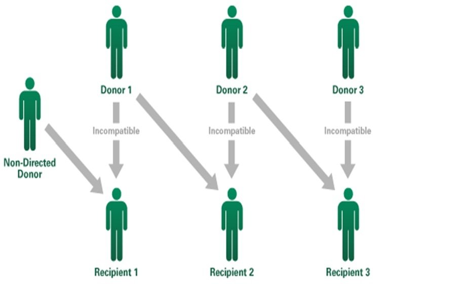
Rees et al. (2009): A Nonsimultaneous, Extended, Altruistic-Donor Chain

Roth et al. (2009): Kidney exchange

Increasing rates of deceased organ donation

Organs from other sources

Shepherd et al. (2014): International comparisons between opt-in vs opt-out systems

Rithalia et al. (2009): The impact of presumed consent

Pierson et al. (2009)

The current status of xenotransplantation

Atala et al. (2009) synthetic organ (bladder) transplantation

Given that there is a shortage of supply...

Our focus is on how to allocate the livers available from deceased donors

Rethinking

deceased donor liver allocation

in the US

Every month over

700

people are added to the liver tx waitlist

In that same month, only

450

people will receive a liver transplant

117,000

people have been listed since 2002

64,000

people have received a liver transplant since 2002

Of those listed since 2002:

21,000

died waiting for a liver

became too sick

got better

15,000

8,000

4,000

living donor

Livers are a precious resource

How should transplant organizations decide how to allocate livers for transplant?

Many possible allocation metrics:

waited longest
shortest survival w/out transplant
longest survival with transplant

benefit the most from transplant
- quality of life
- survival

Keller et al. (2014), Ethical considerations surrounding survival benefit-based liver allocation

Freeman et al. (2014) Who should get a liver graft?

Sickest first: the MELD score

(Model for End-Stage Liver Disease)

Originally designed to predict 3-month transplant-free survival in transjugular intrahepatic portosystemic shunt (TIPS) patients (Malinchoc et al, 2000)

Later deemed useful for estimating prognosis for chronic liver disease (Kamath et al., 2001, 2007)

Adopted by UNOS for liver allocation in 2002

This study was based on 231 patients at 4 US medical centers and validated on 71 patients from the Netherlands

MELD = 10 \times \Big[ 0.957 \log(\textbf{creatinine}) + 0.378 \log (\textbf{bilirubin}) + 1.12 \log (\textbf{INR})\Big] + 6.43

The donor liver is given to the person on the waitlist with the highest MELD score

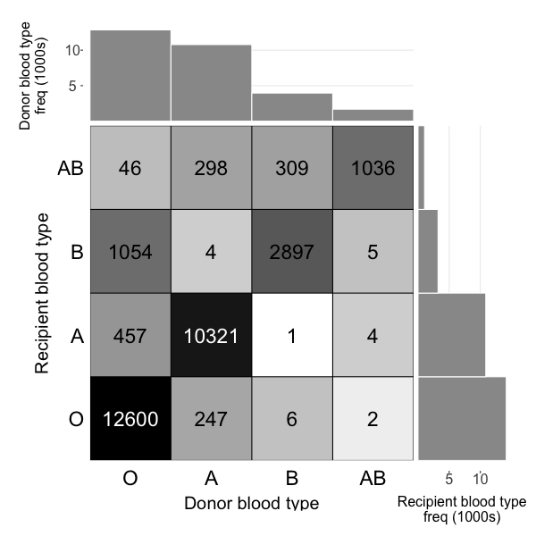
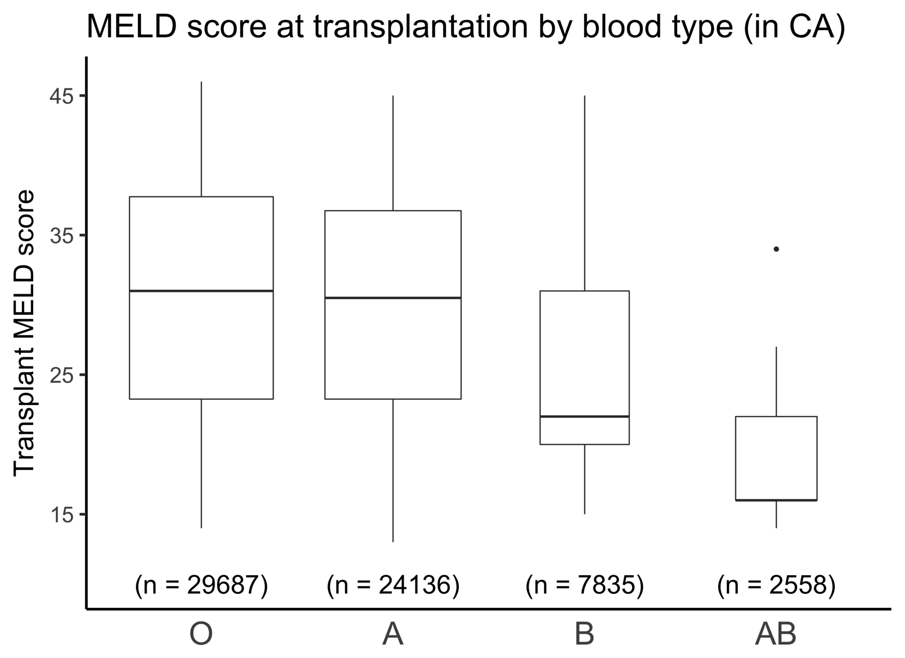
Defining a waitlist:

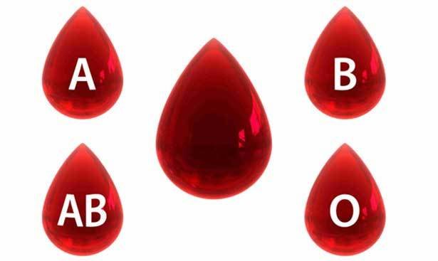
Blood type and Geography

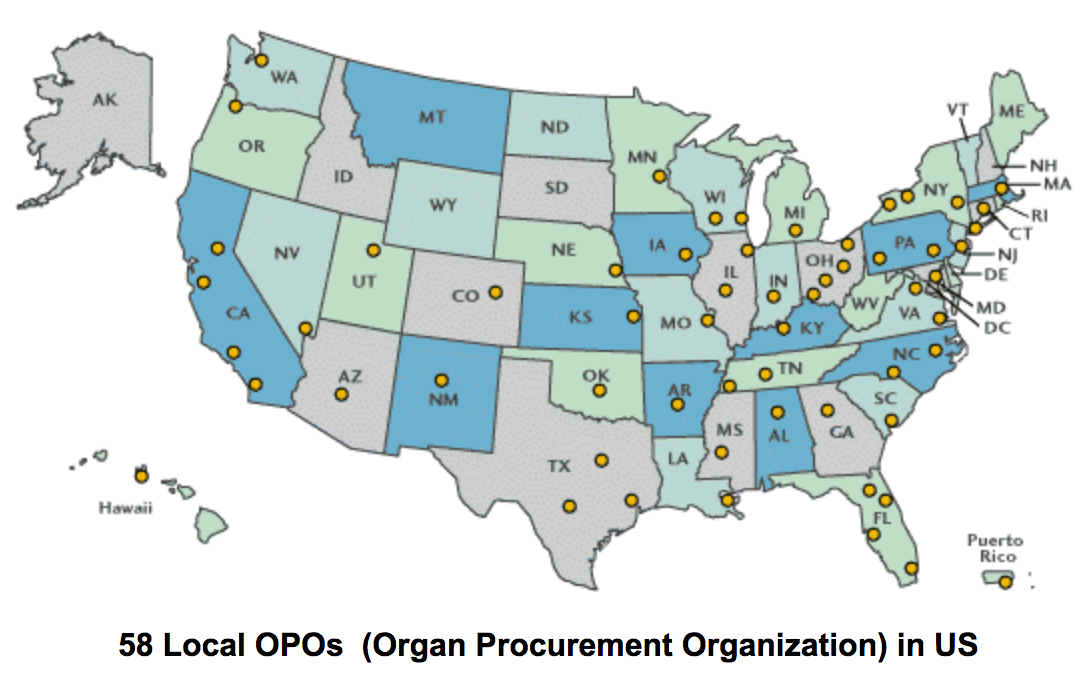
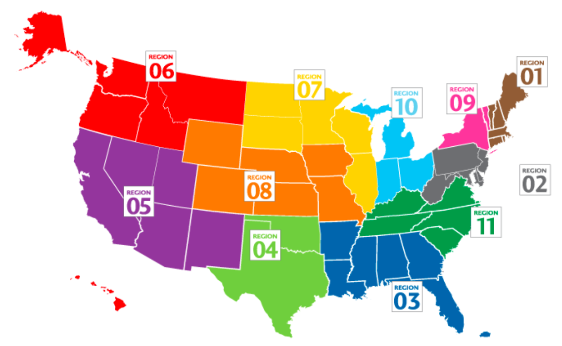
Image source: https://unos.org/transplantation/matching-organs/regions/

Image source: https://sites.google.com/site/esrdandkidneytranpslant/

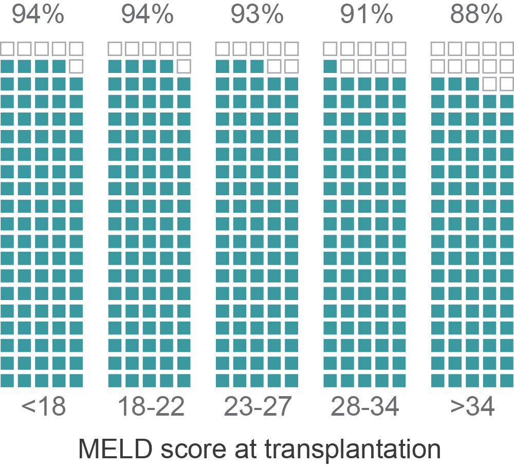
MELD and transplant-free survival

*Data from a single OPO in CA with 3,500 patients and where 85% are transplant-free at 3 months

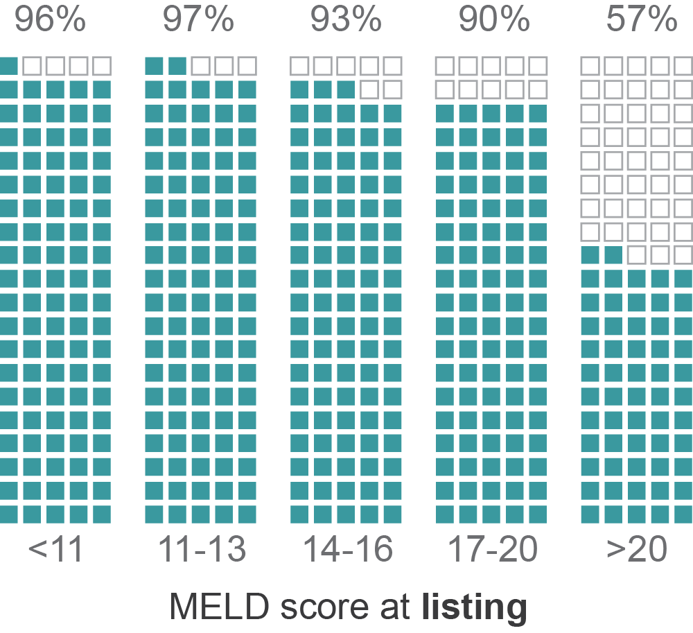
Percent alive at 3 months

(transplant-free)

Criticisms of MELD in the literature

MELD is a poor predictor of post-transplant survival

The current weighting (of INR, bilirubin and creatinine) may not be optimal

MELD should include serum albumin

Meyers et al. (2013), Revision of MELD to include serum albumin improves prediction of mortality on the liver transplant waiting list

Sharma et al. (2008), Re-weighting the model for end stage liver disease score components

Patients with the highest MELD are those with the worst post-transplant outcomes

Klein et al. (2013), Predicting Survival after Liver Transplantation Based on Pre-Transplant MELD Score: a Systematic Review of the Literature

Siparsky et al. (2014), Organ allocation in liver transplantation

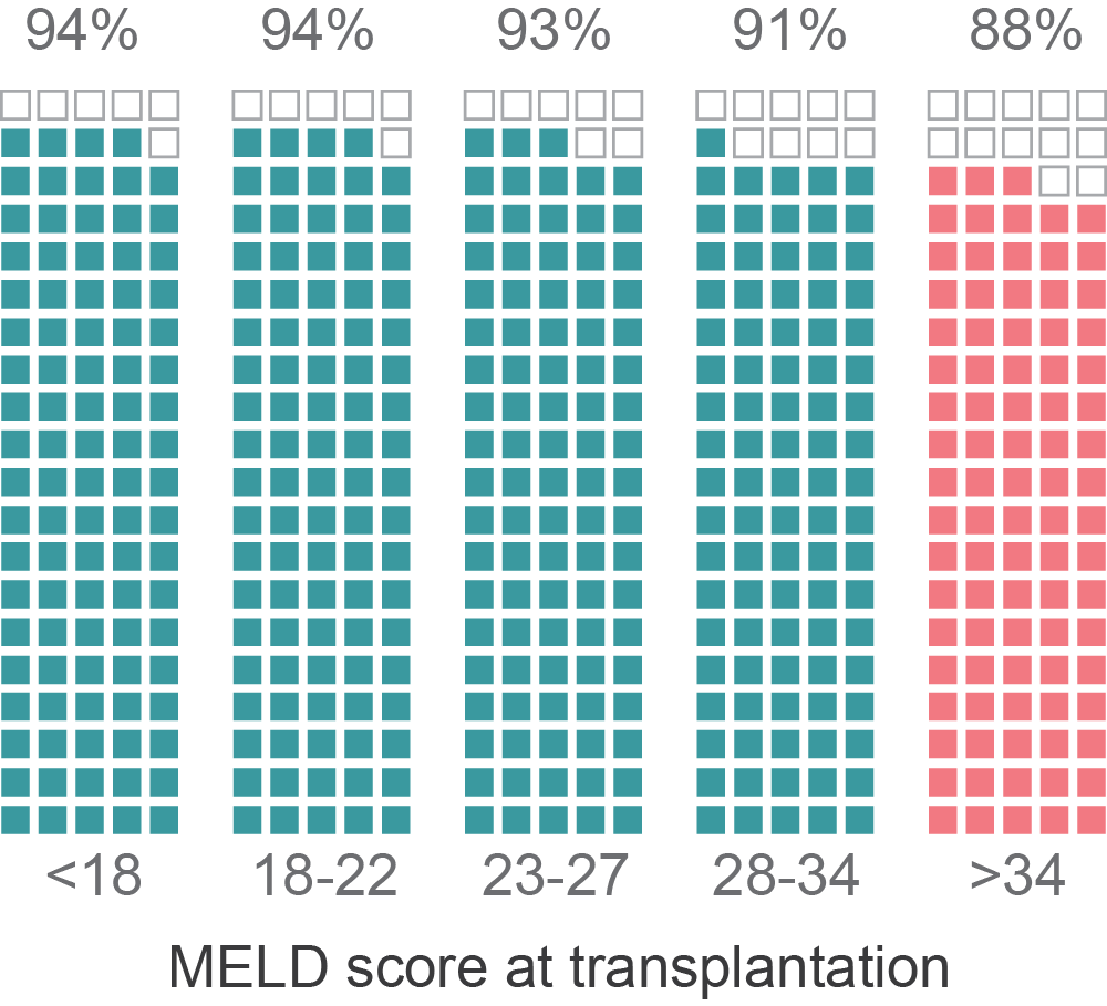
Percent alive at 6 months (post-transplant)

transplantation

Estimating transplant benefit

Defining transplant benefit

benefit

survival with a transplant

survival without

a transplant

Fundamental problem of causal inference:

We can only observe one!!!

Existing approaches to estimating benefit

Control outcome

(censored)

Treated

outcome

11/01/2003

Control outcome

(observed)

Merion et al. (2005)

Shaubel et al. (2009)

Difference between 5-yr predicted survival for two Cox models

Single Cox model with transplant indicator

Deals with censoring using inverse probability of censoring weighting (Robins and Finkelstein, 2000)

Do not address bias from censoring

Informative censoring:

Earlier censoring = higher and/or more rapidly increasing MELD score

Confounding:

Difference in MELD score between control and treatment

Merion et al. (2005), Shaubel et al. (2009)

Do not address potential confounding

The data isn't really designed to compare transplanted versus untransplanted...

Transplanted

first

Transplanted

last

With the UNOS data, we are far from a random experiment:

Sickest

Healthiest

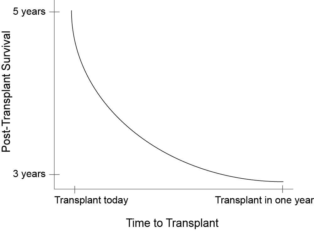
Our approach: redefining transplant benefit

Redefining our causal effect

Consider the causal effect on survival of

increasing wait time to transplantation

(i.e. receiving a transplant now vs later)

In 2 weeks

In one year

In 2 months

4 yrs

3.5 yrs

3 yrs

What is t = 0?

A specific MELD score, e.g. first time MELD is 18

Redefining our causal effect

If we could observe the outcome of all possible wait times for an individual...

Unfortunately we only observe one point on the individual's curve

Maybe we can populate the curve with observations with other similar patients

The problem is that patients with a shorter wait time tend to be sicker...

Sickness is a confounder!

Can we find features of the data that allow us to do comparisons across wait times that are "as if random"?

Exploiting randomness in the data

Two sources of randomness in wait times

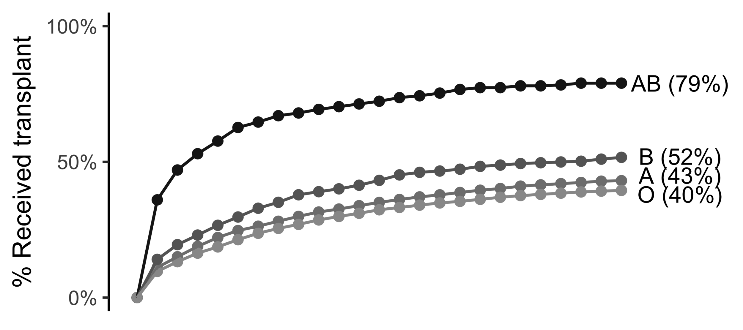
Wait time differs by blood type

(Universal donor)

(Universal recipient)

A quick foray into instrumental variables

Instrumental Variables

\textrm{dead in 1yr}_i = \beta_0 + \beta_1 \textrm{(tx in 1mo)}_i + ~~...~~ + \epsilon_i

terms we can control for

terms we can't control for

(e.g. future MELD)

Correlated

AB is 23% more likely than O to be transplanted in 1 month

AB is 7% less likely than O to die within 1 year

Causal effect of tx in 1mo on death in 1yr:

\frac{\textrm{Effect of AB on death in 1yr}}{\textrm{Effect of AB on tx in 1mo}} = \frac{-0.07}{0.23} = -0.30

Exclusion restriction!

Imbens & Angrist (1994), Identification and estimation of local average treatment effects

Exclusion restriction

The instrument affects the outcome only through the treatment

Blood type B is correlated with higher life expectancy (Shimizu et al (2004))
Blood type B is correlated with lower life expectancy (Brecher et al. (2015))
No correlation between blood type and life expectancy (Vasto (2011))

Research on link between blood type and race:

Research on link between life expectancy and race:

This matches what the literature says...

O'Neil (2001), Modern Human Variation: Distribution of Blood Types

Research on direct link between blood type and life expectancy:

Lots of literature showing a correlation between race and life expectancy

Thielke et al. (2015) Sex, Race, and Age Differences in Observed Years of Life, Healthy Life, and Able Life among Older Adults in The Cardiovascular Health Study
Cantu et al. (2014) New estimates of racial/ethnic differences in life expectancy with chronic morbidity and functional loss: evidence from the National Health Interview Survey

Other assumptions

Relevance of instrument

Monotonicity

SUTVA

Exchangeability of instrument

The treatment assignment of an individual has no effect on the potential outcomes of any other individual

The instrument has a nonzero effect on the instrument

The instrument has a monotonic effect on the treatment across the population. I.e. it either always increases or does not change (but never decreases) the probability of treatment

The instrument does not share any common causes with the outcome (possibly after conditioning on observed covariates)

Two-stage least squares

\textrm{dead in 1yr}_i = \alpha + \beta \textrm{(tx in 1mo)}_i + ... + \epsilon_i

Two stage least squares estimation of :

\beta

Stage 1: regress the treatment on the instrument

\textrm{(tx in 1mo)}_i = \gamma_0 + \gamma_1 \textrm{A}_i + \gamma_2 \textrm{B}_i + \gamma_3 \textrm{AB}_i + \gamma_4 \textrm{OPO}_i + \gamma_5 \textrm{ethnicity}_i + \nu_i

instruments

(blood type dummies)

Stage 2: regress the outcome on the predicted treatment

\textrm{(dead in 1yr)}_i = \beta_0 + \beta_1 \textrm{(tx in 1mo)}_i + \beta_2 \textrm{OPO}_i + \beta_3 \textrm{ethnicity}_i + \epsilon_i

predicted treatment

(from first stage)

treatment

outcome

Things get complicated when trying to adapt to survival models

(Terza et al. 2008, Wan et al. (2015), Cai et al. (2011), Tchetgen Tchetgen et al. (2015))

IV as Two-stage least squares

\hat{\beta}_{2SLS} = \frac{Cov(Y, ~\hat{T})}{Var(\hat{T})}

= \frac{Cov(Y, ~\gamma_0 + \gamma_1Z)}{Var(\gamma_0 + \gamma_1 Z)}

=\frac{1}{\gamma_1} \frac{ Cov(Y, Z)}{ Var(Z)}

= \frac{Var(Z)}{Cov(T, Z)} \frac{Cov(Y, Z)}{Var(Z)}

= \frac{Cov(Y, Z)}{Cov(T, Z)}

= \hat{\beta}_{IV}

T_i = \gamma_0 + \gamma_1 Z_i + \nu_i

Y_i = \beta_0 + \beta_{2SLS} \hat{T}_i + \epsilon_i

Y_i = \omega_0 + \omega_1 Z_i + \epsilon_i

\hat{\beta}_{IV} = \frac{\omega_1}{\gamma_1}

2SLS

IV (Wald)

T_i = \gamma_0 + \gamma_1 Z_i + \nu_i

A sequential IV approach

(that doesn't deal with hazard models!)

IV for survival outcomes

Survival models

\textrm{wait time}_i = \gamma_0 + \gamma_1 \textrm{A}_i + \gamma_2 \textrm{B}_i + \gamma_3 \textrm{AB}_i + \gamma_4 \textrm{OPO}_i + \gamma_5 \textrm{ethnicity}_i+ \nu_i

Stage 1: OLS to predict wait time

Tchetgen Tchetgen et al. (2015) Instrumental variable estimation in a survival context

Cox model is non-collapsable:

Use an additive model instead

(estimate the marginal causal effect on hazard of transplantation one week earlier)

Stage 2: Additive hazard model (predictor substitution)

\lambda(t) = \beta_0(t) + \beta_1 \textrm{(wait time)} + \beta_2 \textrm{OPO}_i(t) + \beta_3 \textrm{ethnicity}_i(t) + \epsilon_i(t)

(Alt) Stage 2: Additive hazard model (residual inclusion / control function)

\lambda(t) = \beta_0(t) + \beta_1 \textrm{(wait time)} + \beta_2\Big( \textrm{(wait time) - (wait time)} \Big)

+ \beta_3 \textrm{OPO}_i(t) + \beta_4 \textrm{ethnicity}_i(t) + \epsilon_i(t)

Results show that Predictor Substitution is inconsistent but residual inclusion is consistent.(Terza et al. (2008), Wan et al. (2015), Cai et al. (2011))

Results

Marginal causal effect on hazard of waiting one extra week for a transplant

Residual inclusion estimate:

0.000000867 (-0.000000878, 0.00000325)

Residual inclusion estimate:

0.000000832 (-0.000000137, 0.00000322)

A sequential IV approach

(MELD 18)

Month (t)

A = (0, 0, 1, 1, 1, 1, 1, 1, 1)

Y = (0, 0, 0, 0, 1, 1, 1, 1, 1)

A = (0, 0, 0, 0, 0, 0, 0, 0, 0)

Y = (0, 1, 1, 1, 1, 1, 1, 1, 1)

A = (0, 0, 0, 0, 0, 1, 1, 1, 1)

Y = (0, 0, 0, 0, 0, 0, 0, 0, 0)

A = (0, 0, 0, 0, 0, 0, 0, 0, 0)

Y = (0, 0, 0, 0, 0, 0, 0, 0, 0)

A = (0, 0, 0, 1, 1, 1, 1, 1, 1)

Y = (0, 0, 0, 0, 0, 0, 0, 0, 0)

A = (0, 0, 0, 0, 0, 0, 0, 0, 0)

Y = (0, 0, 0, 0, 0, 0, 0, 0, 0)

2SLS (1)

Y = death by month 1

A = tx by month 1

Z = blood type

2SLS (3)

Y = death by month 3

A = tx by month 3

Z = blood type

2SLS (2)

Y = death by month 2

A = tx by month 2

Z = blood type

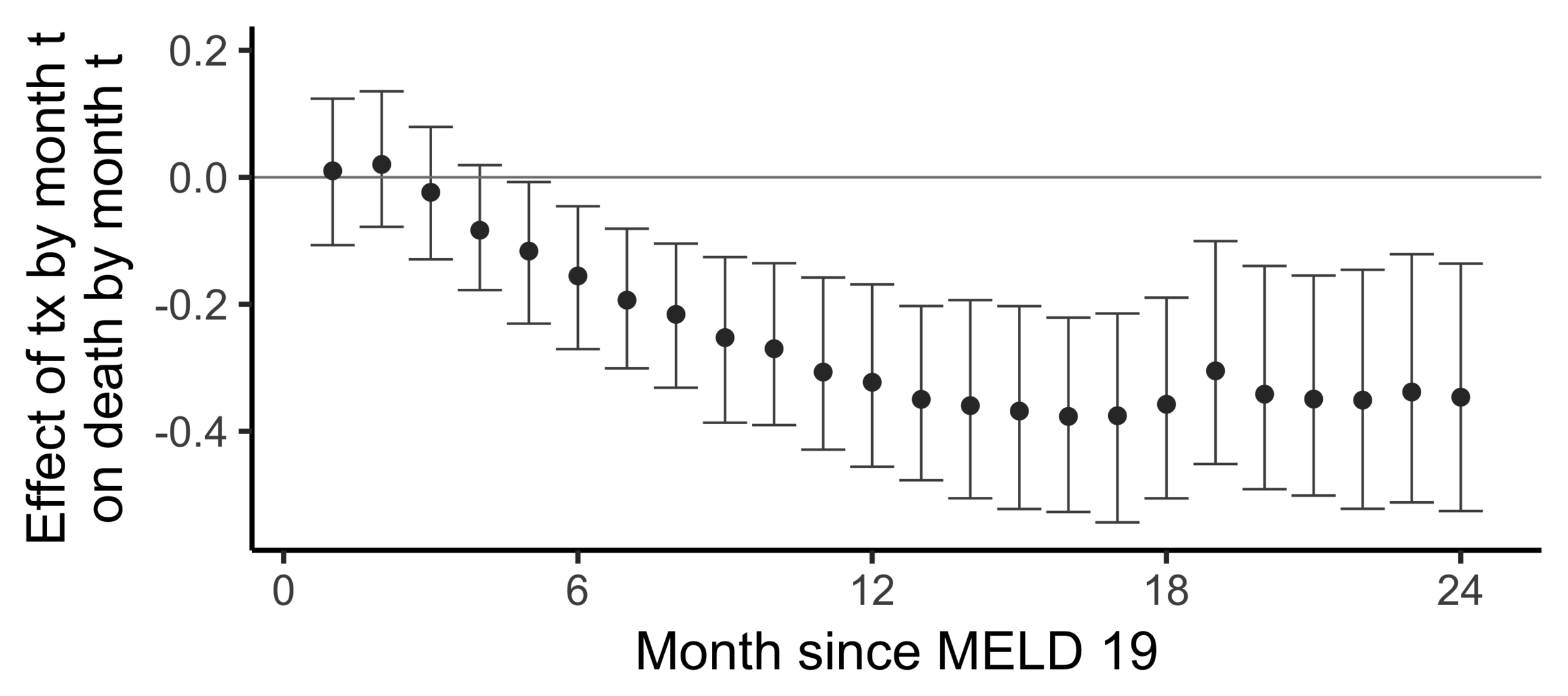
The effect of receiving a transplant...

The effect on death by 24 months

receiving a transplant by 24 months

versus

not having receiving a transplant yet

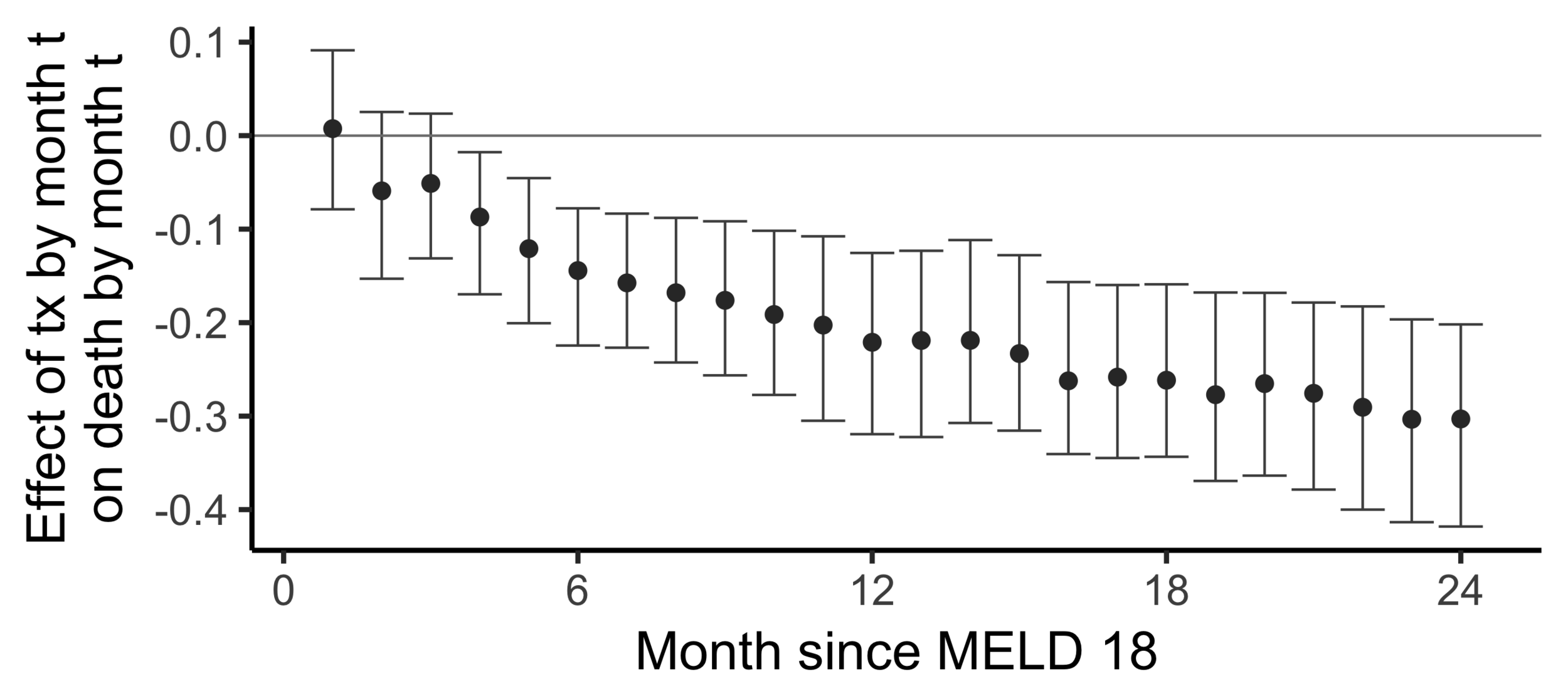
(\textrm{Death by 24mo})_i = \alpha + \beta (\textrm{tx by 24mo})_i + \epsilon_i

(2SLS estimate)

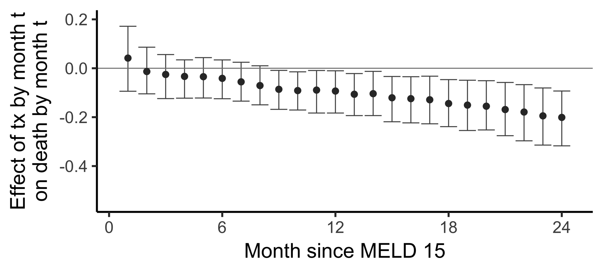
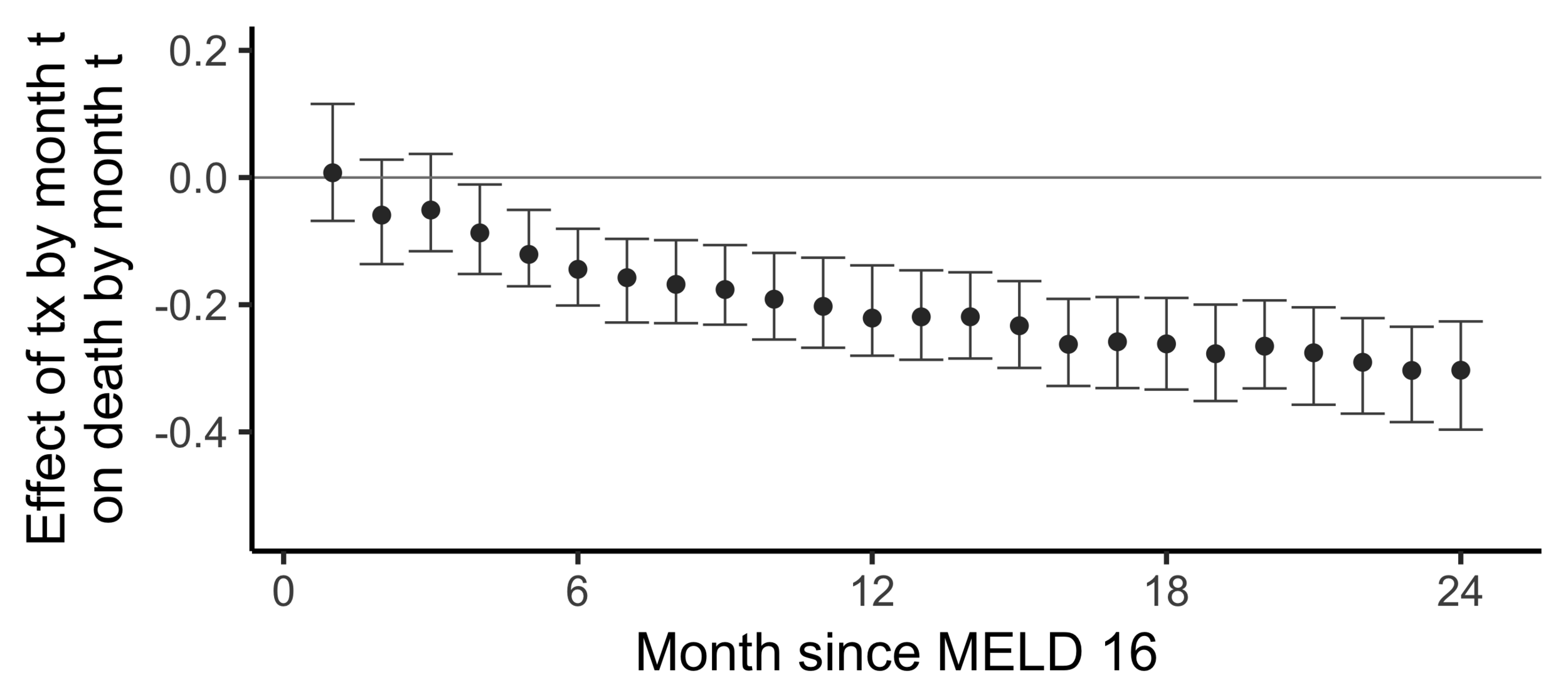
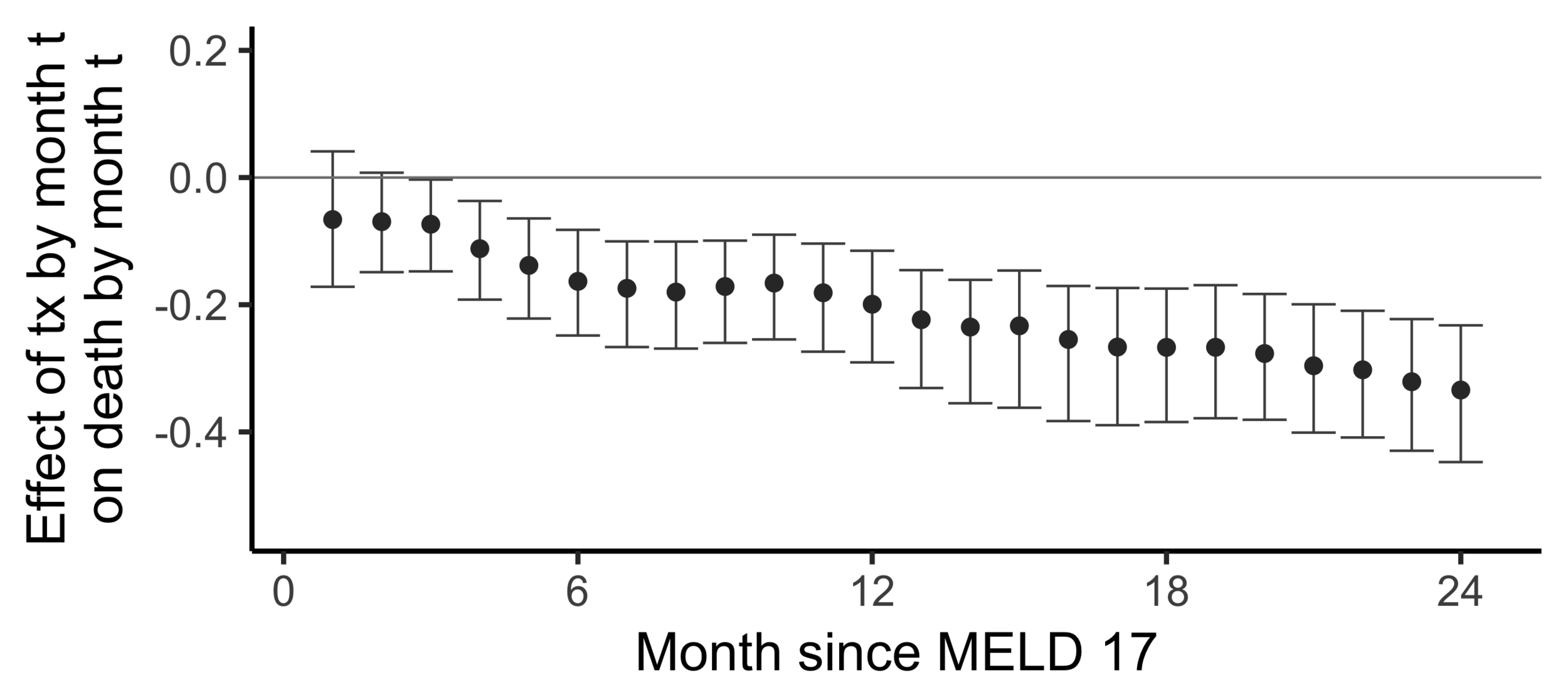
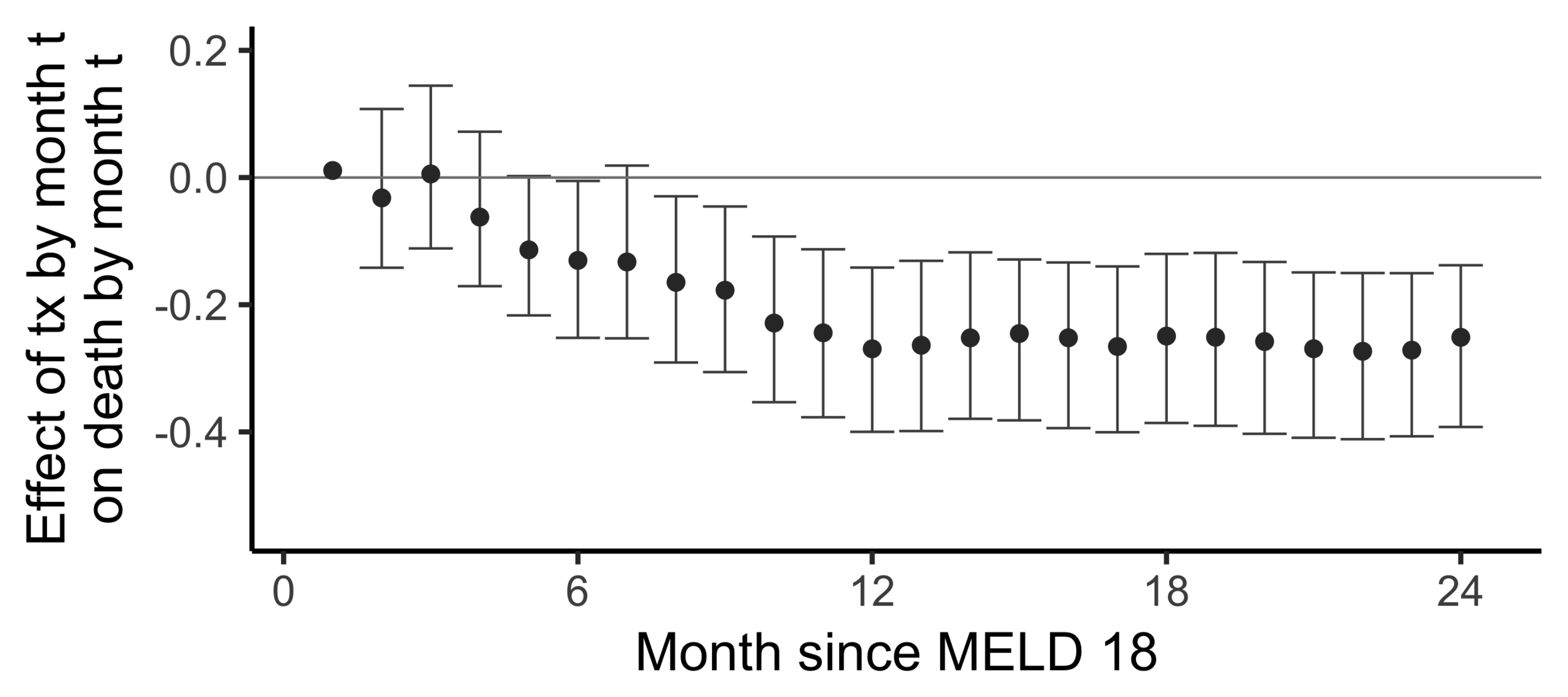
Subsampling stability

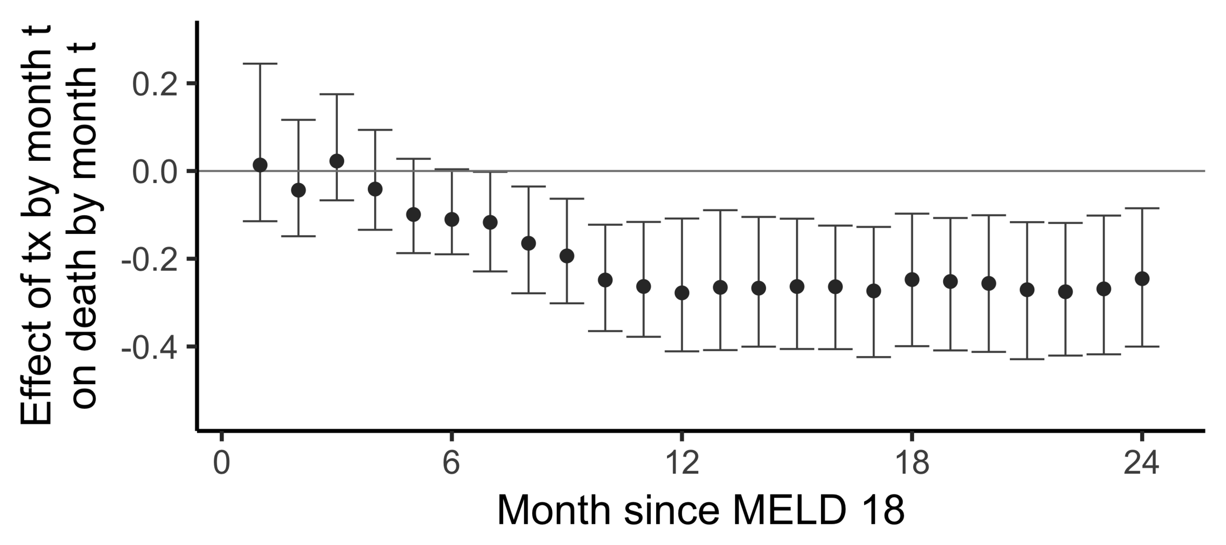
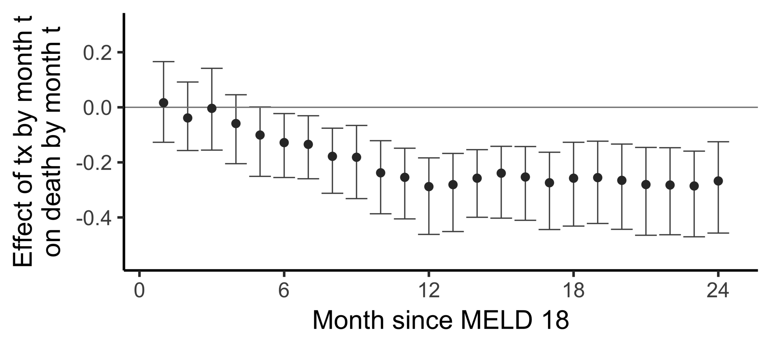
Stability with respect to MELD

A sequential non-parametric approach

(MELD 18)

Month (t)

A = (0, 0, 1, 2, 3, 4, 5, 6, 7)

Y = (0, 0, 0, 0, 1, 1, 1, 1, 1)

A = (0, 0, 0, 0, 0, 0, 0, 0, 0)

Y = (0, 1, 1, 1, 1, 1, 1, 1, 1)

A = (0, 0, 0, 0, 0, 1, 2, 3, 4)

Y = (0, 0, 0, 0, 0, 0, 0, 0, 0)

A = (0, 0, 0, 0, 0, 0, 0, 0, 0)

Y = (0, 0, 0, 0, 0, 0, 0, 0, 0)

A = (0, 0, 0, 1, 2, 3, 4, 5, 6)

Y = (0, 0, 0, 0, 0, 0, 0, 0, 0)

A = (0, 0, 0, 0, 0, 0, 0, 0, 0)

Y = (0, 0, 0, 0, 0, 0, 0, 0, 0)

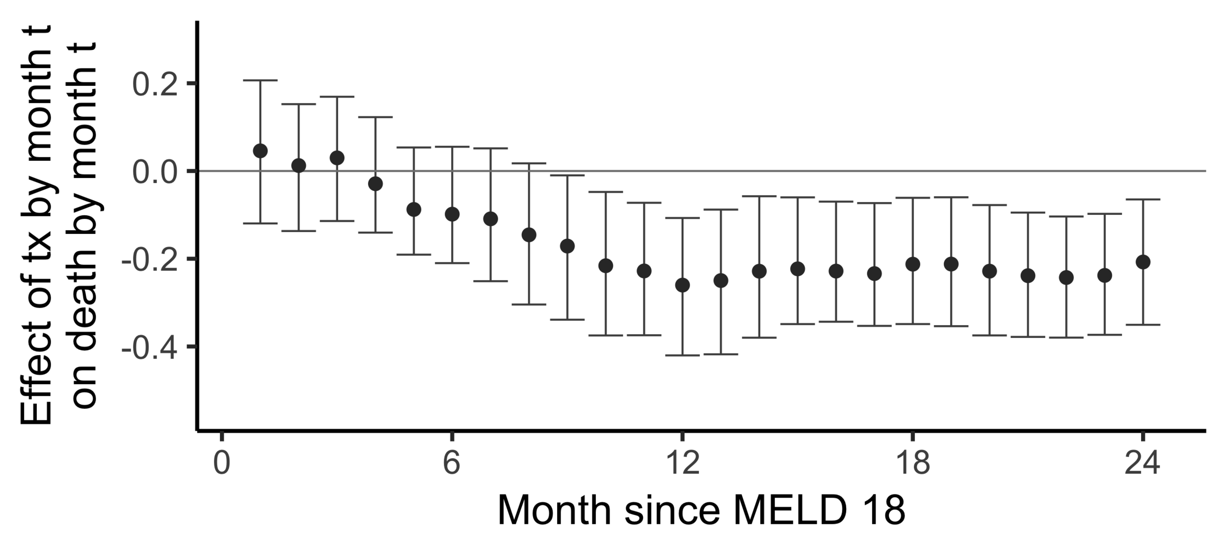
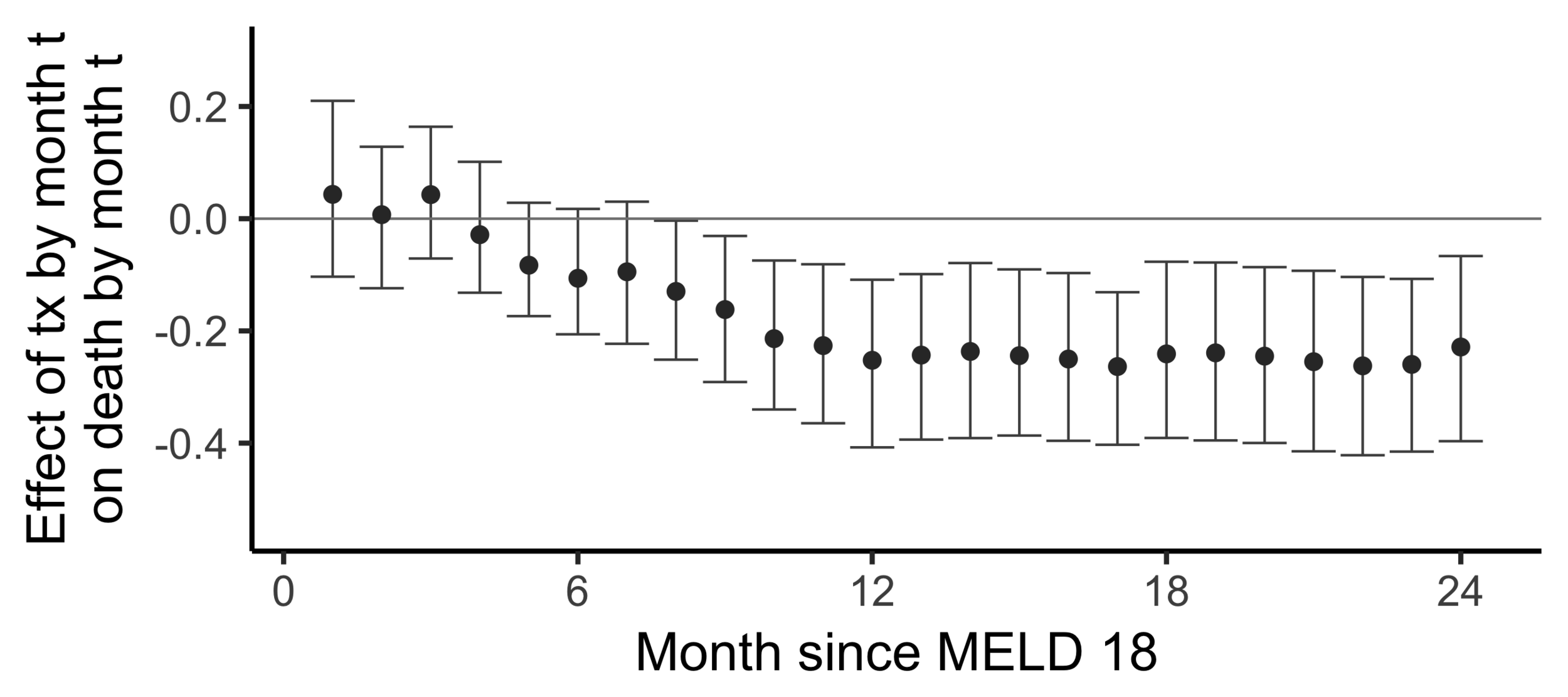
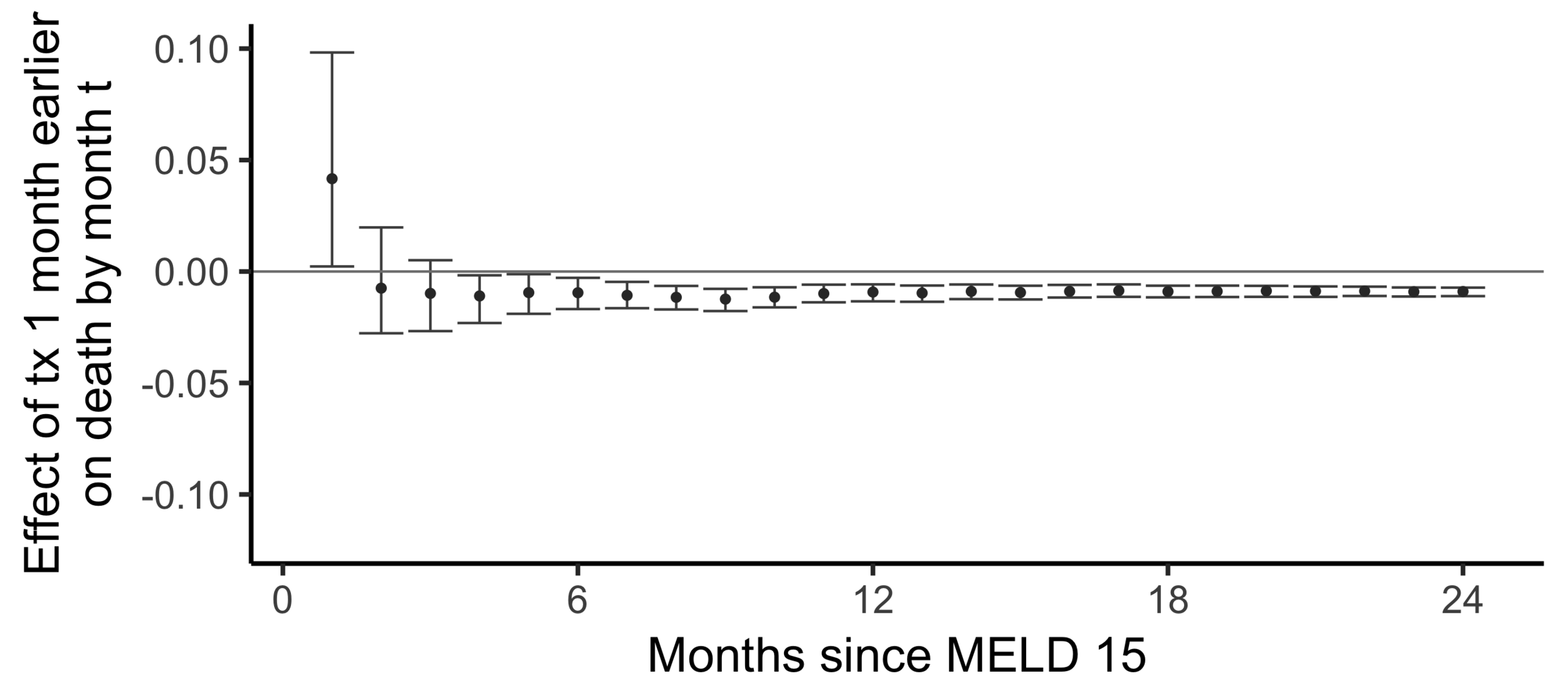
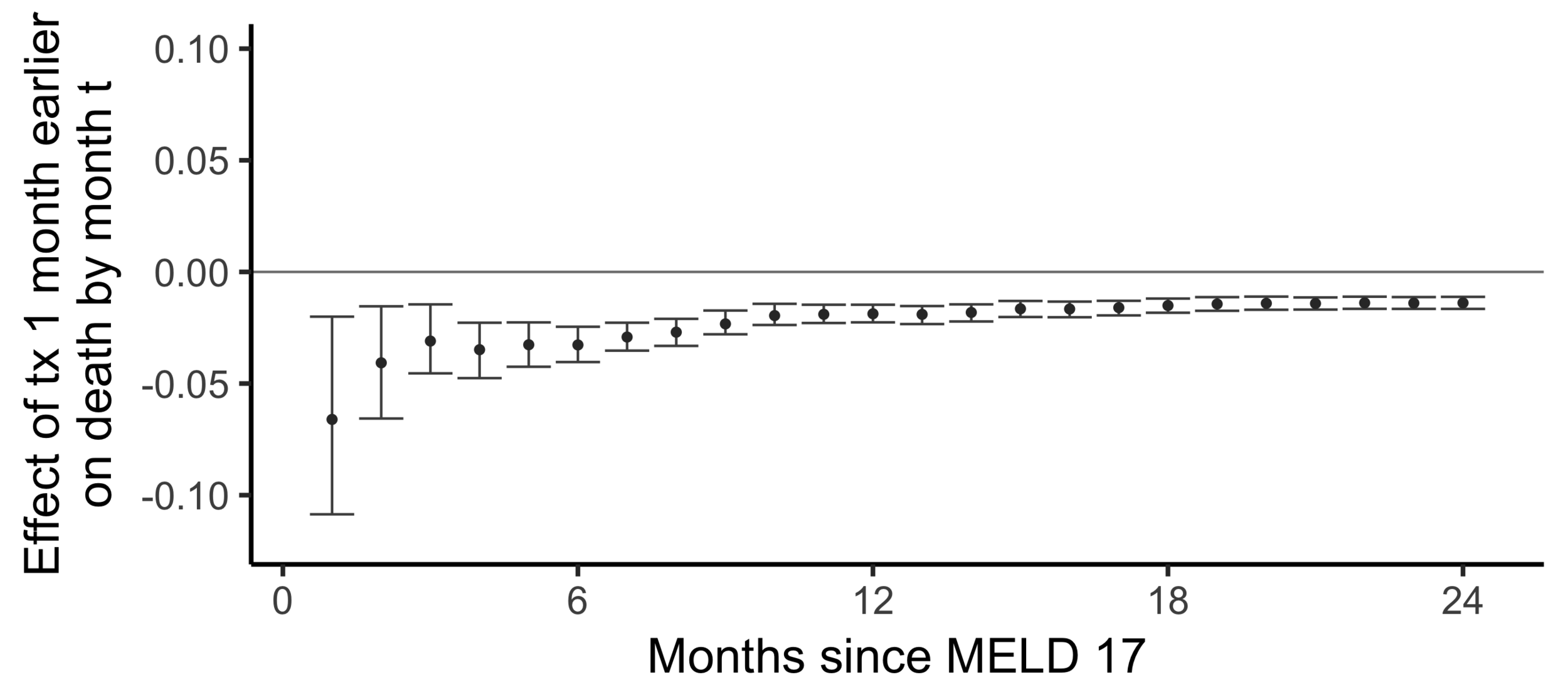
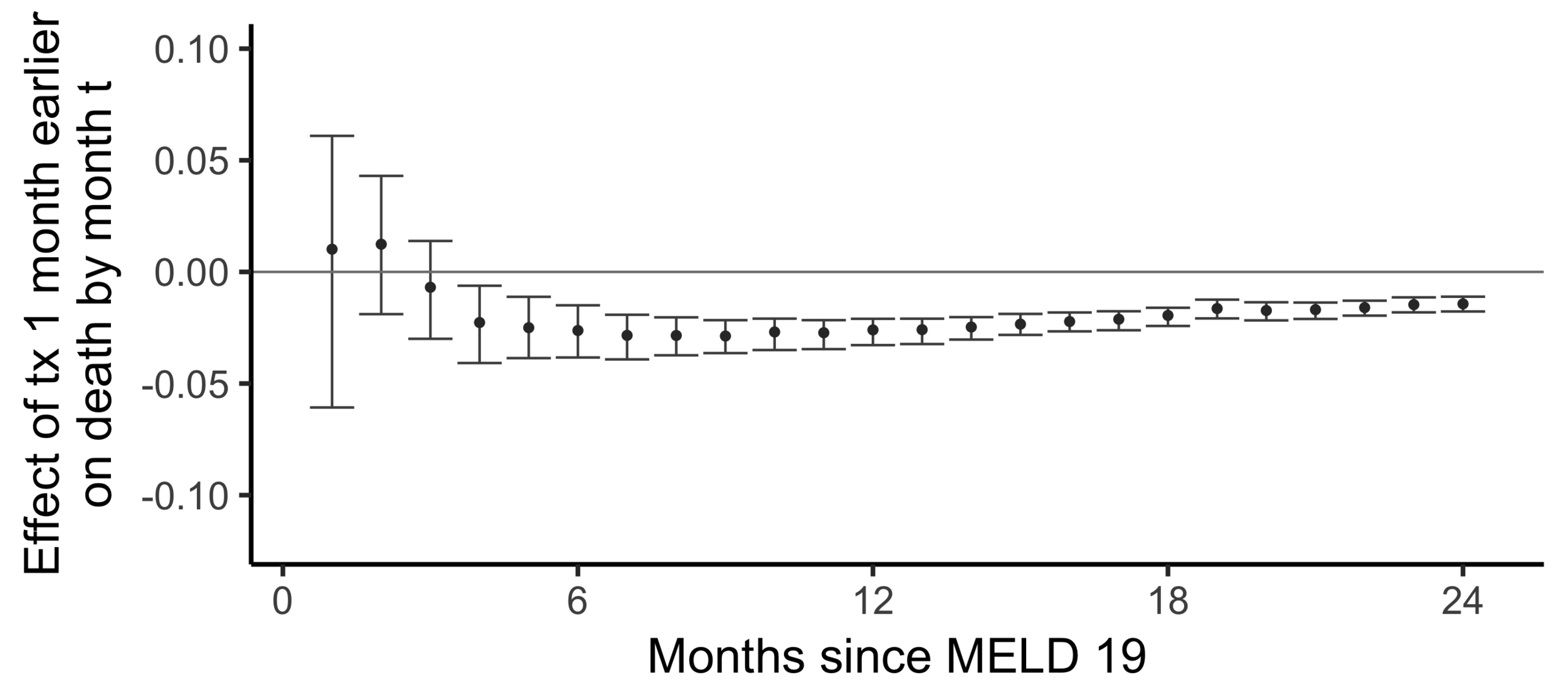
The effect on death by month 24

being transplanted one month earlier than actually transplanted

(\textrm{Death by 24mo})_i = \alpha + \beta (\textrm{months since tx})_i + \epsilon_i

Effect on the chance of death by 24 months of being transplanted 6 months earlier:

-0.014 \times 6 = -8.4\%

-0.014 -

The effect of receiving a transplant earlier

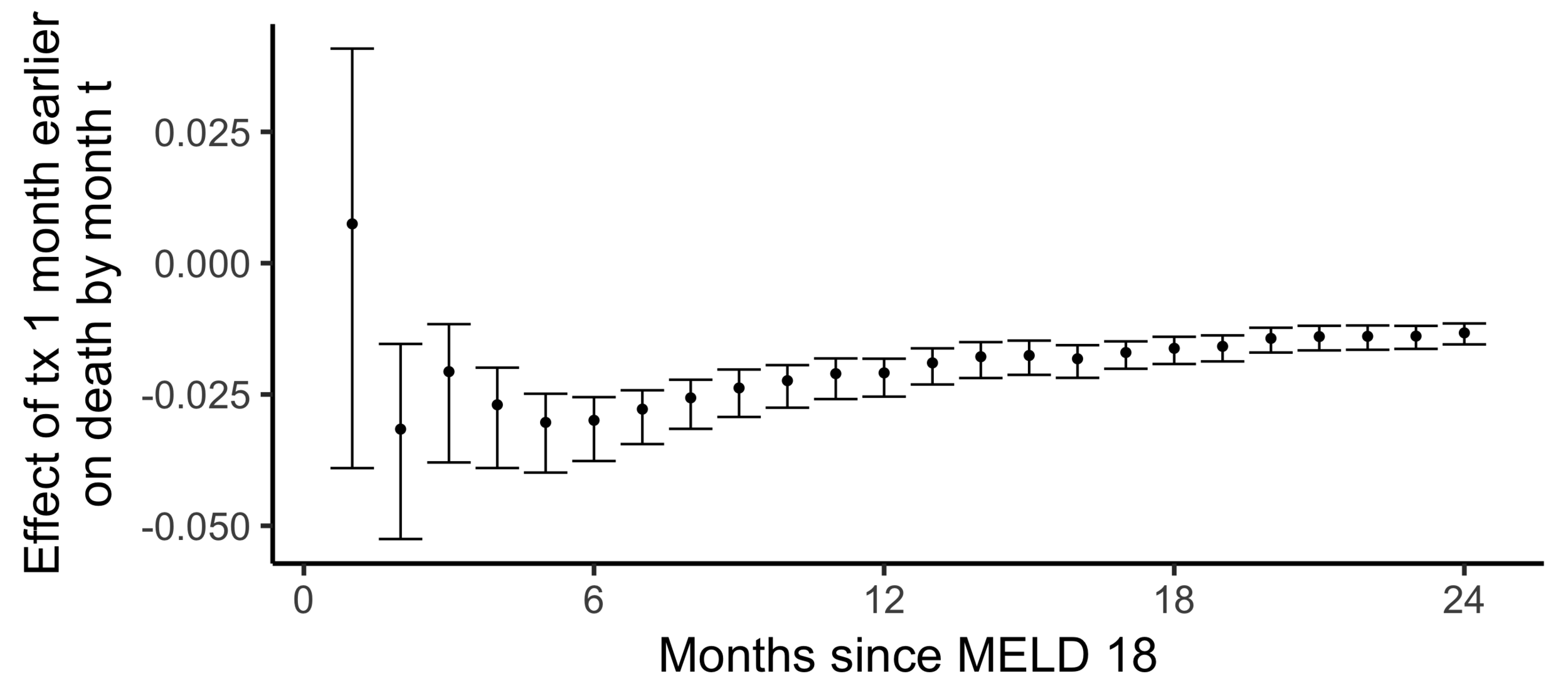
(2SLS estimate)

Subsampling stability

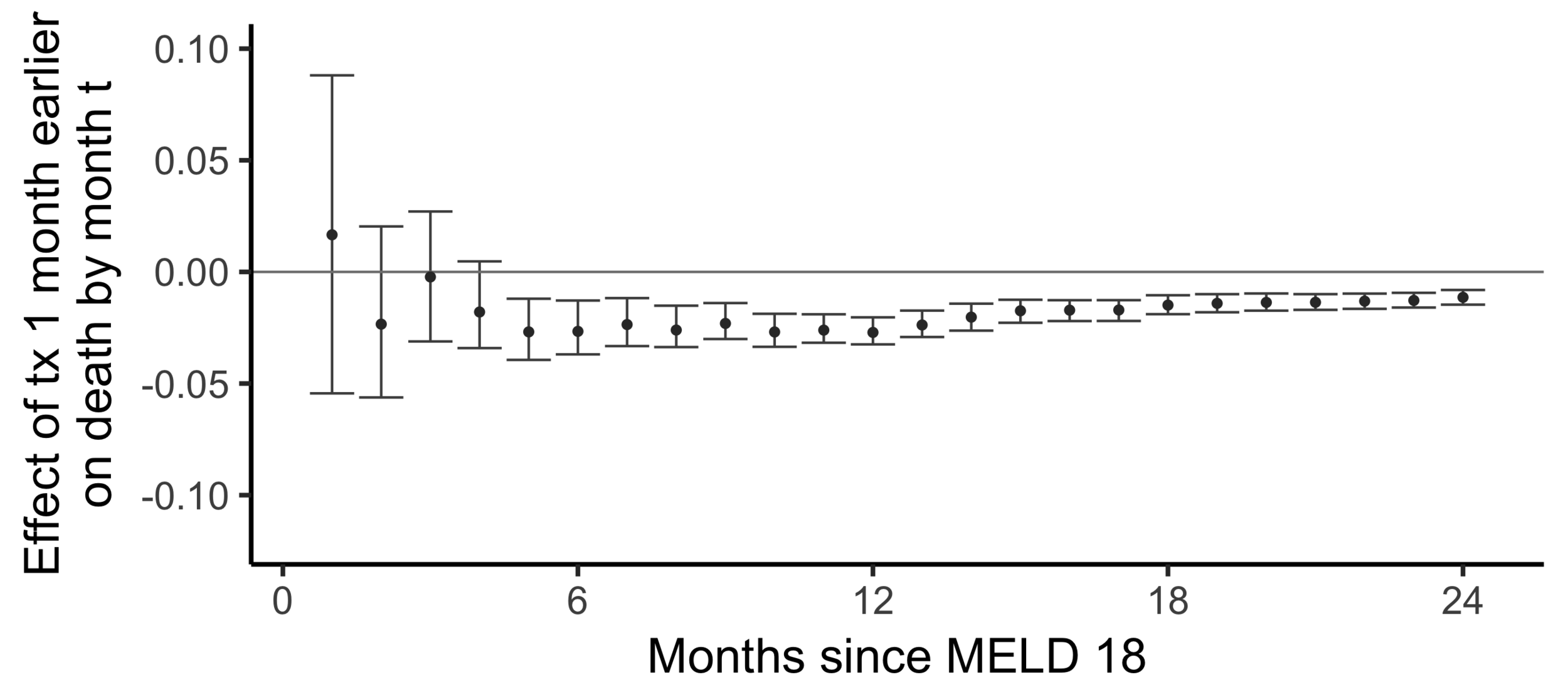
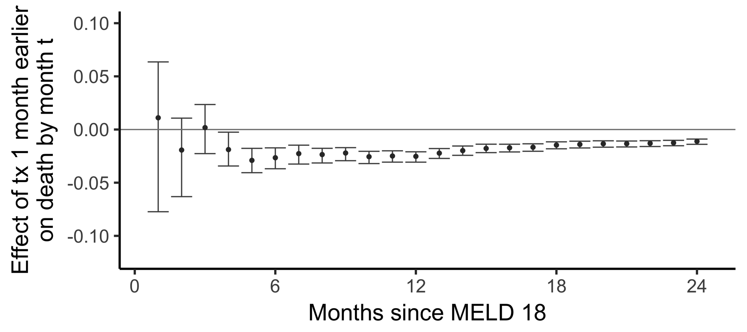
Stability with respect to MELD

Comparing wait times by state

Wait time differs by state

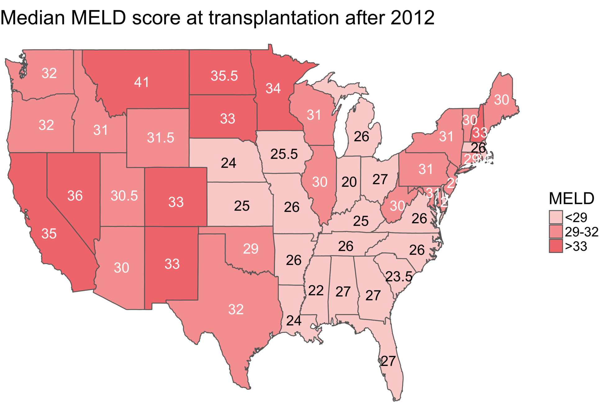
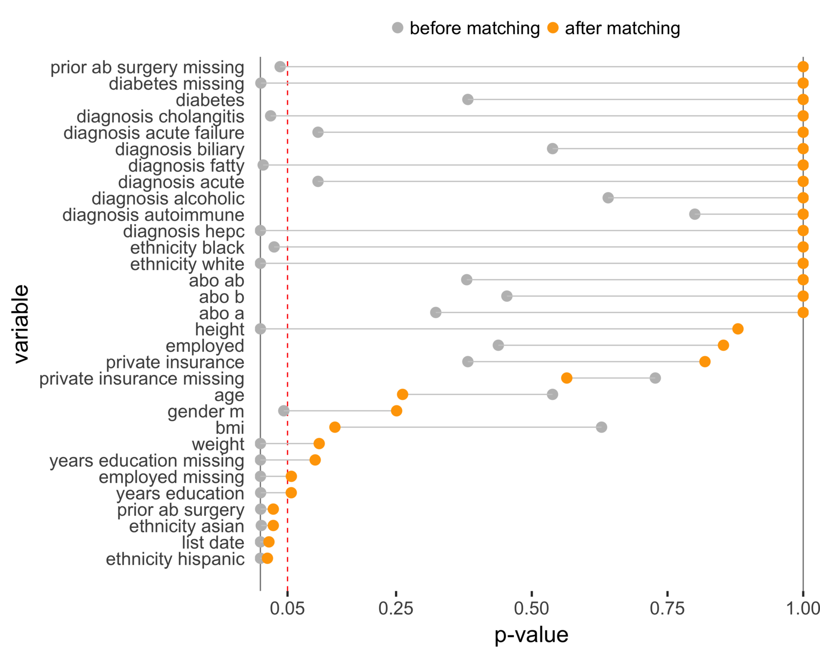
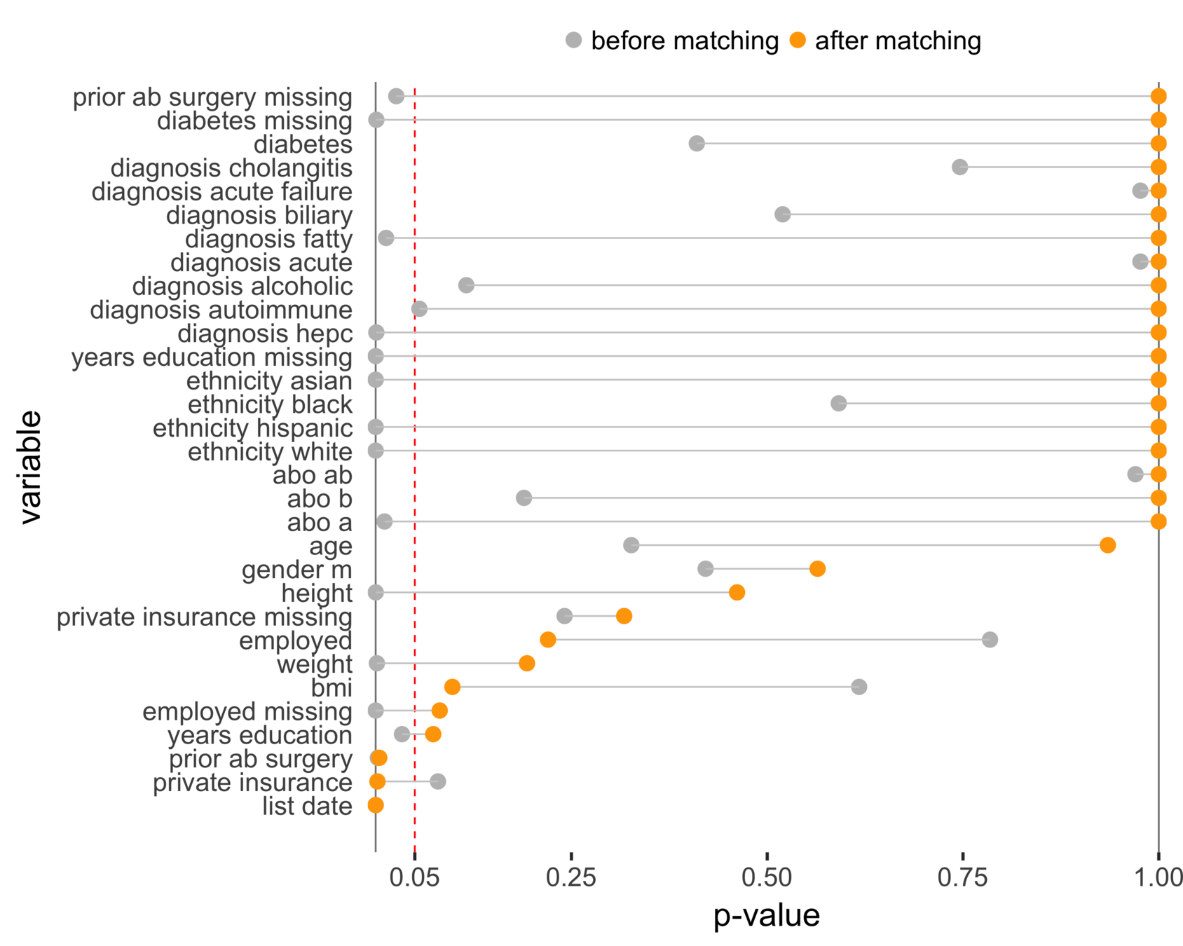
Matching CA and NC

Sekhon (2011), Multivariate and Propensity Score Matching Software with Automated Balance Optimization: The Matching Package for R

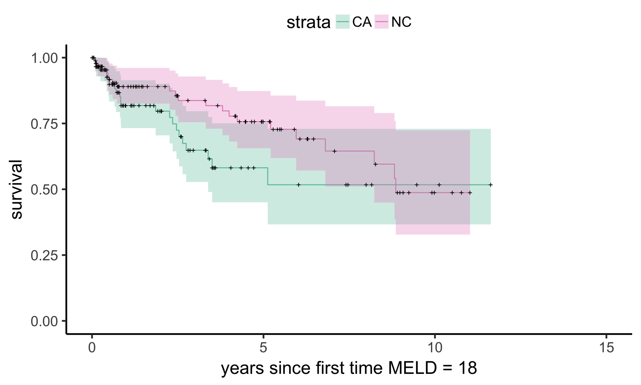
CA (MELD 38)

NC (MELD 24)

Matching CA (n = 686) to NC (n = 150)

Balance (NC & CA)

Stability: equivalent comparisons

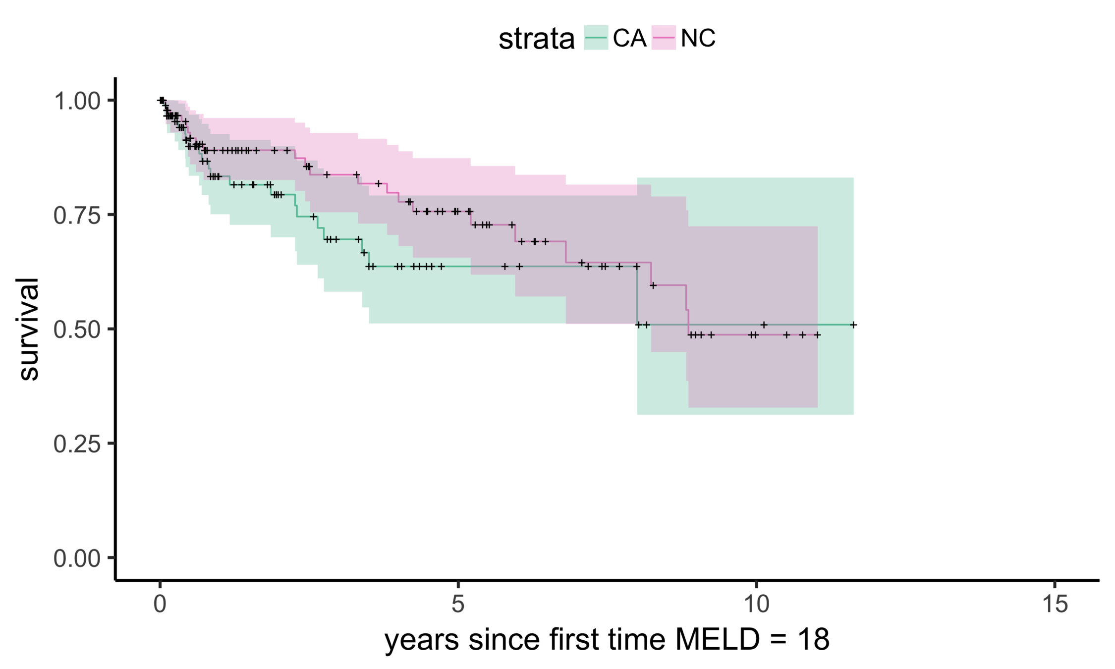
CA (MELD 38)

OH (MELD 24)

Matching CA (n = 686) to OH (n = 195)

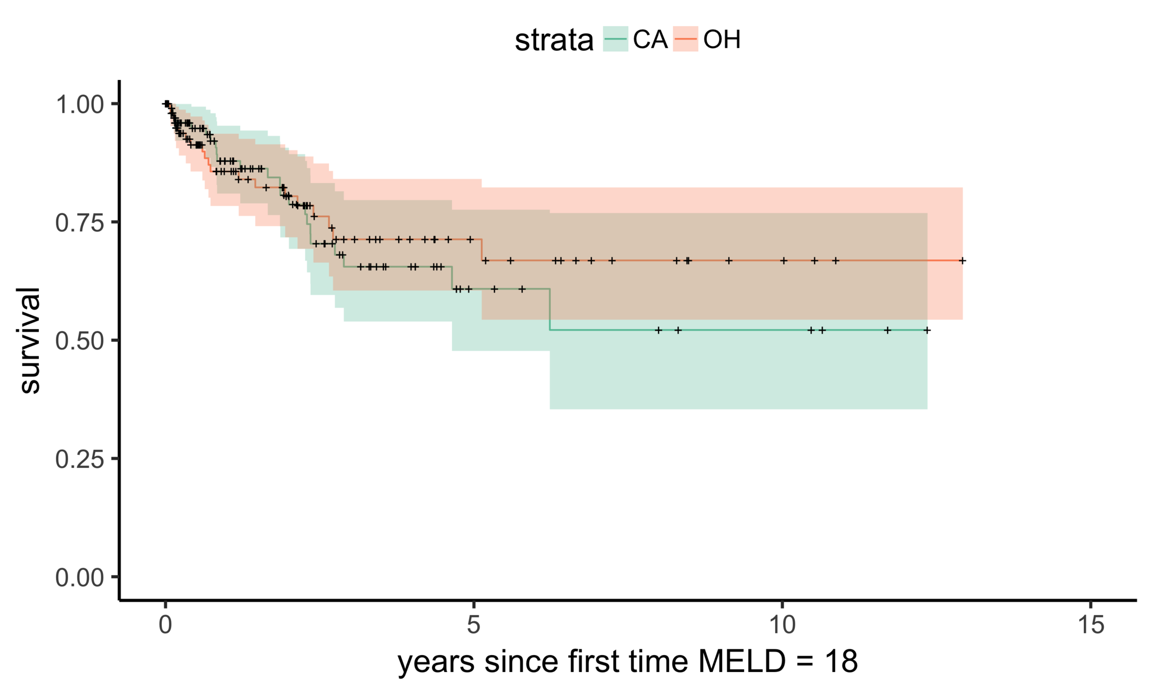
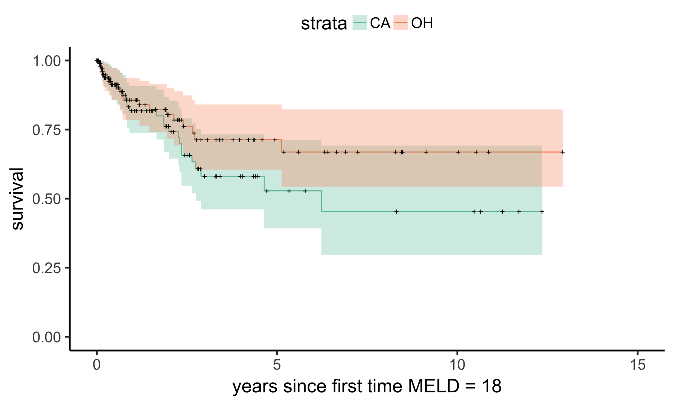
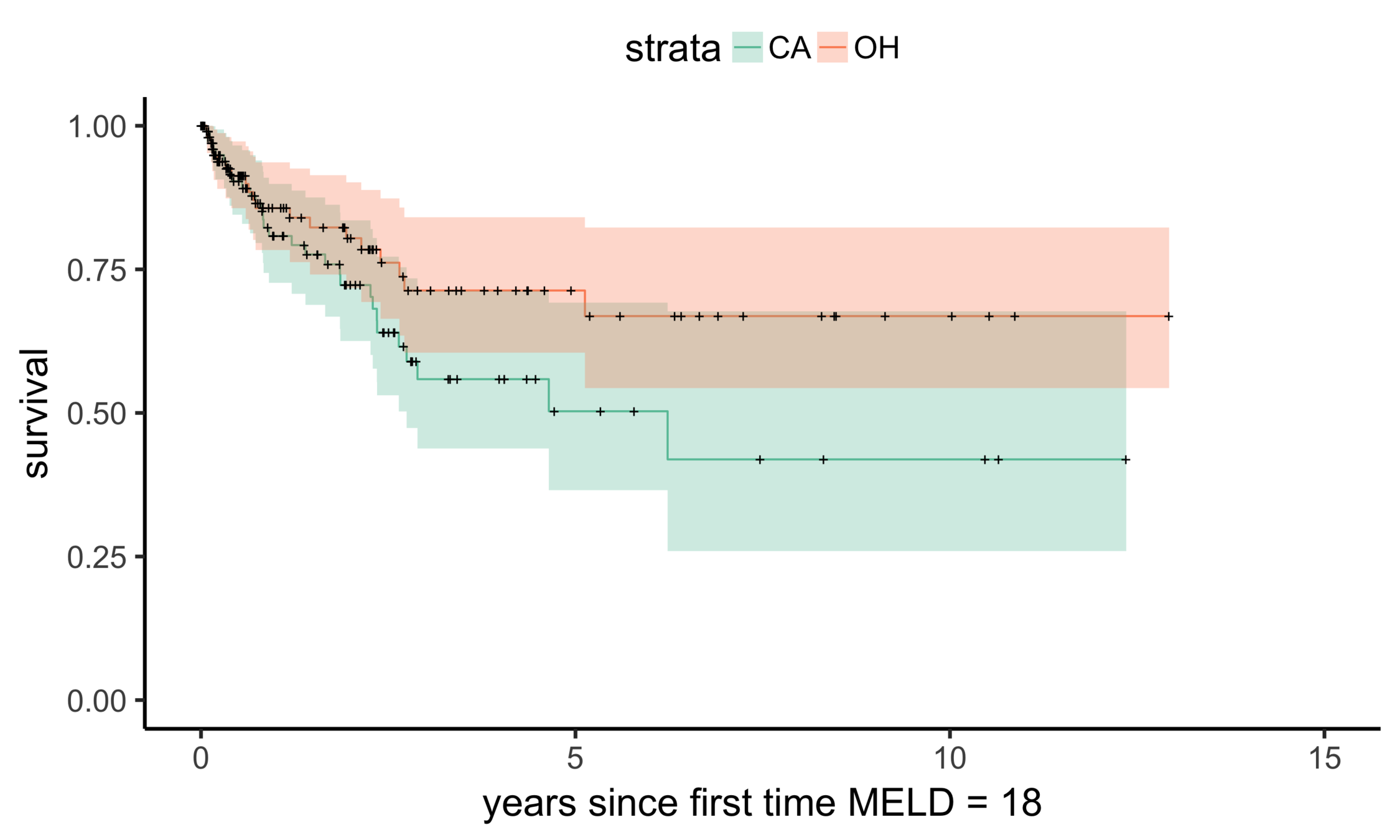
Balance (CA & OH)

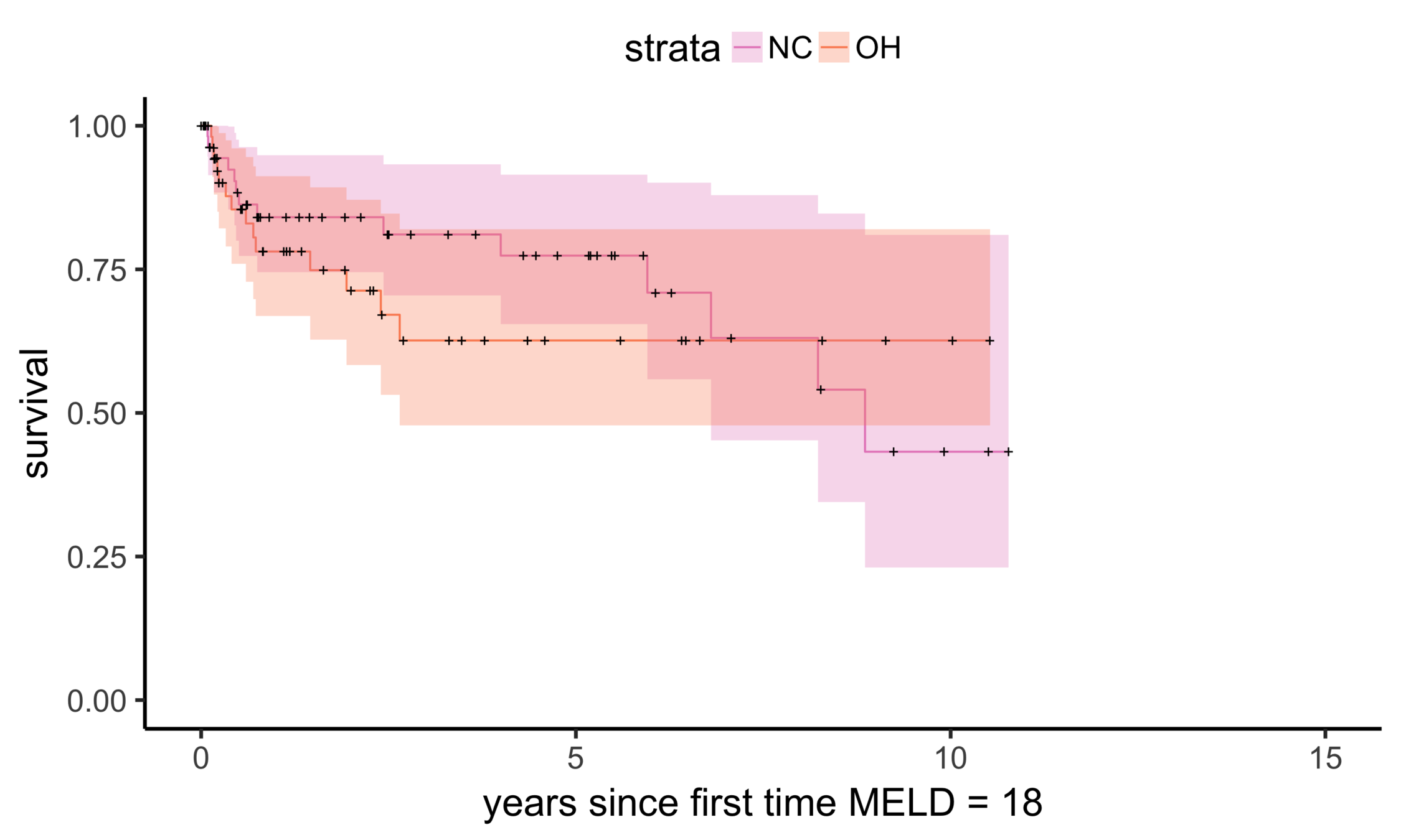
Stability: null comparisons

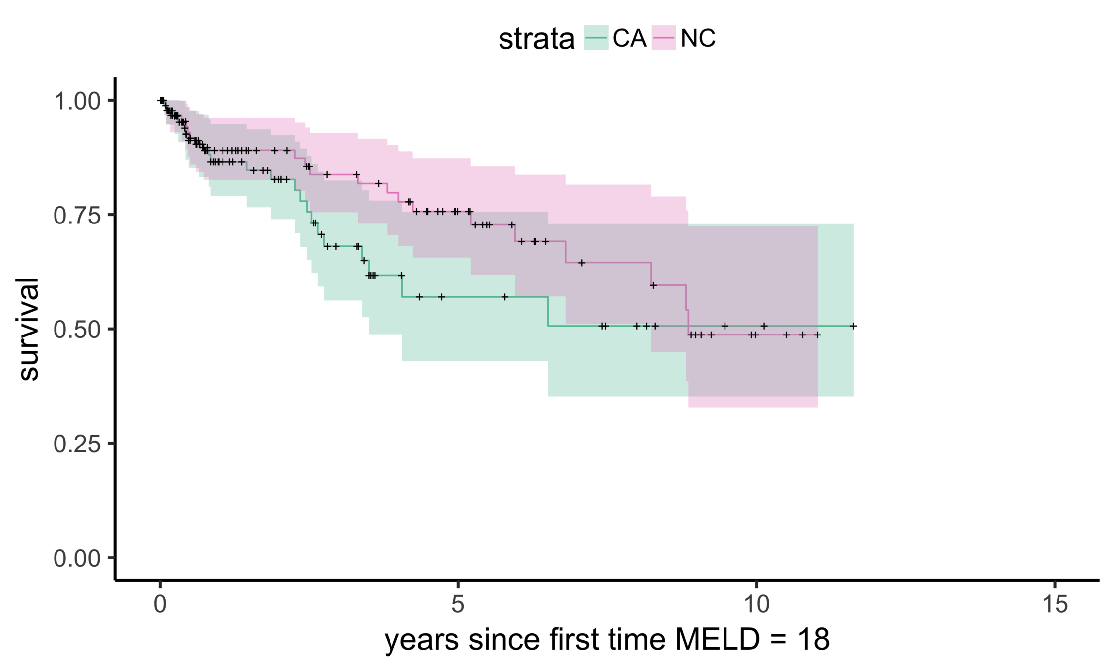
NC (MELD 24)

OH (MELD 24)

Matching OH (n = 195) vs NC (n = 150)

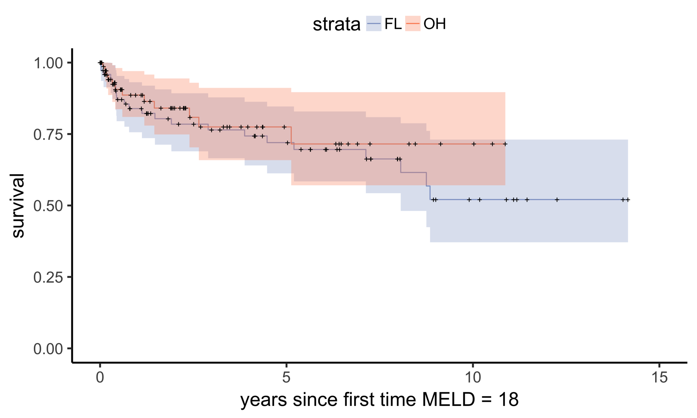
OH (MELD 24)

FL (MELD 24)

Matching OH (n = 195) vs FL (n = 305)

Recap

A = (0, 0, 1, 1, 1, 1, 1, 1, 1)

Y = (0, 0, 0, 0, 1, 1, 1, 1, 1)

What did we learn?

It is very difficult to quantify the effect of transplantation wait time on survival.

Results imply a benefit of being transplanted sooner rather than later.

Where next (UNOS)?

Is there a considerable benefit in being transplanted sooner? For who? How much?

What is the best way to estimate benefit for current patients on the waitlist?

Should allocations policies be altered? If so, how?

Can we estimate benefit on quality of life?

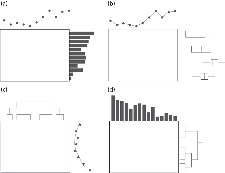
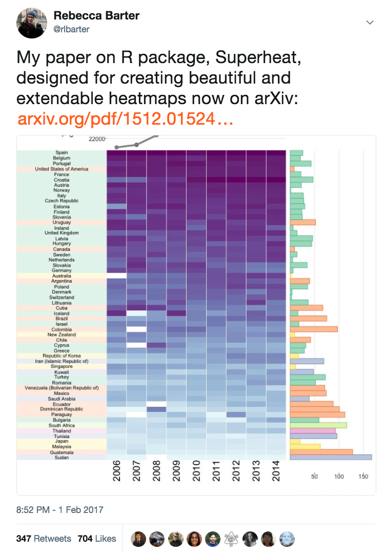
Superheat

package

an

Heatmaps

Trakhtenberg et al. (2016) Cell types differ in global coordination of splicing and proportion of highly expressed genes

Clustering &

Dendrogram

Wilkinson (1994)

Eisen et al. (1998)

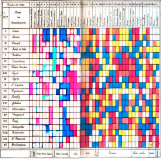
Loua (1873), Atlas statistique de la population de Paris

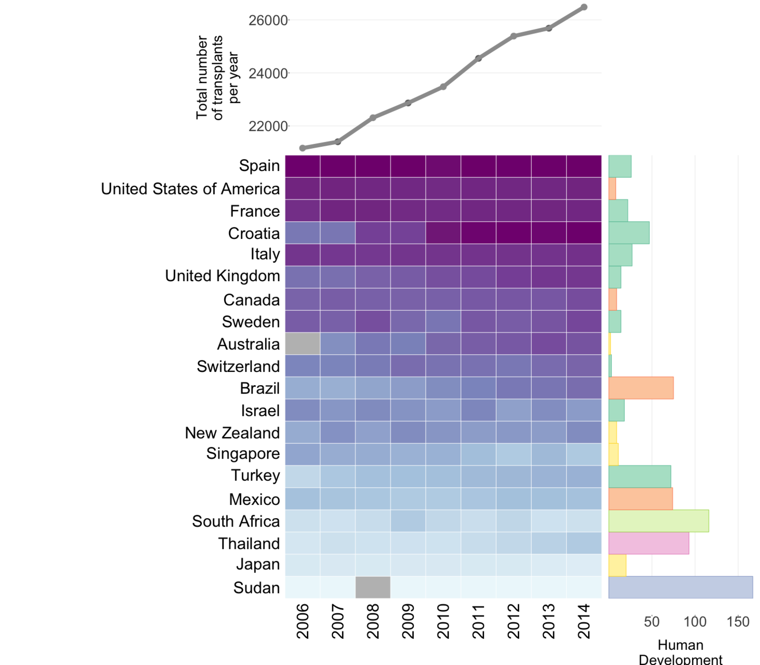
Global organ donation trends over time

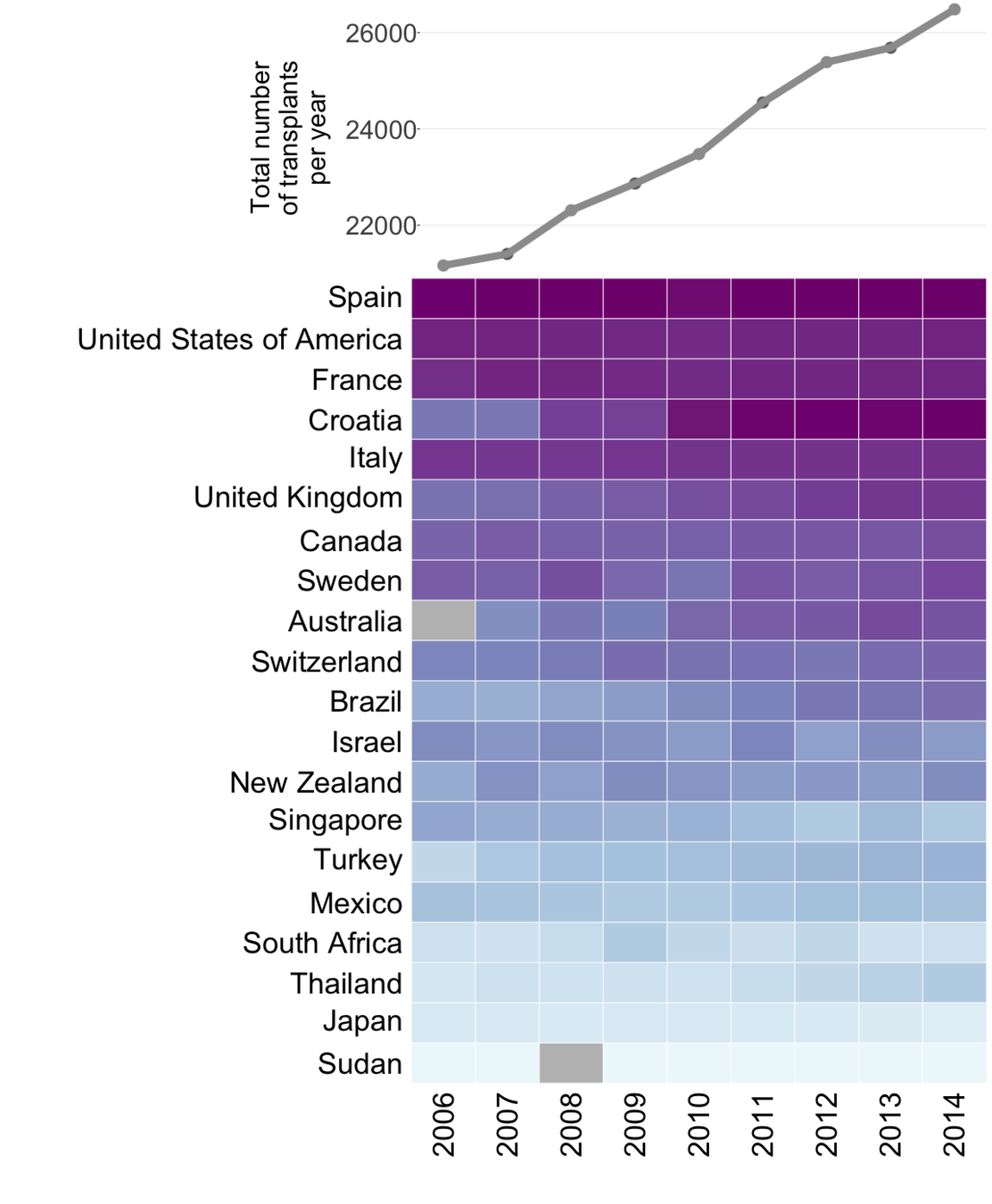
Organ donation trends

with a trendline

and

human development

index ranking

Visualizing lawyer's ratings on US Supreme Court judges

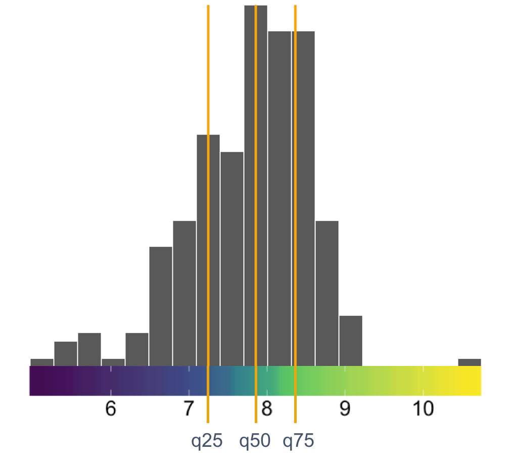
A linear color map

A manual color map

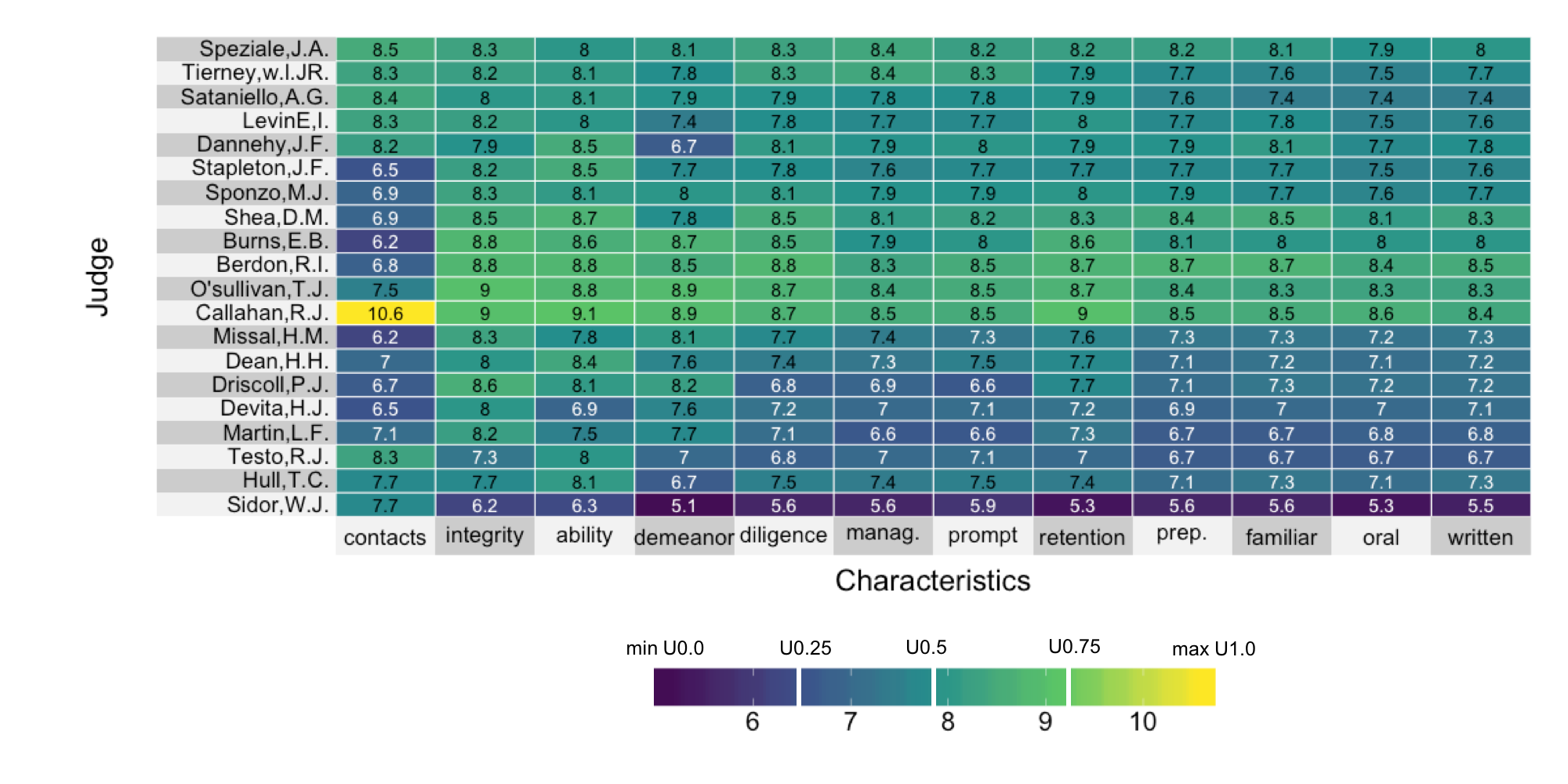
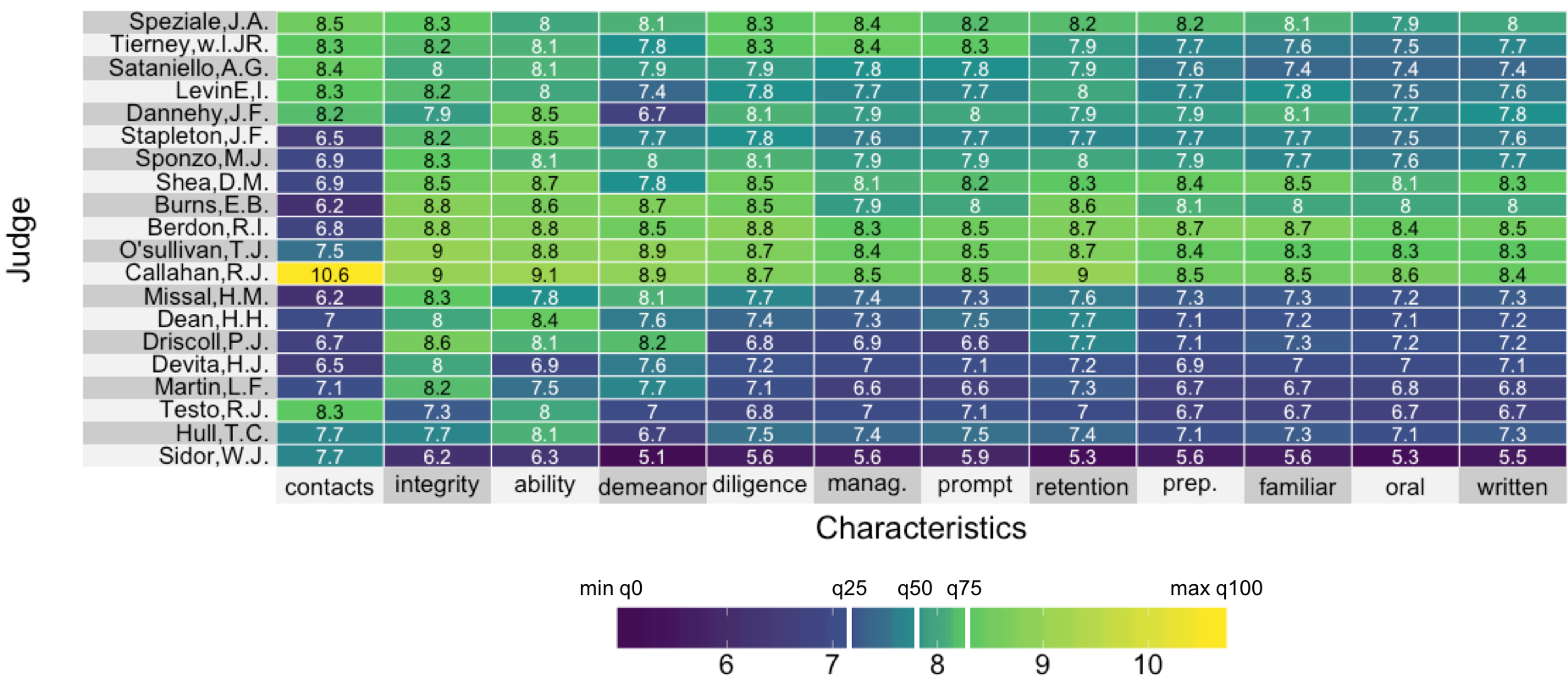
A quantile color map

uperheat success!

Where next (PhD)?

(Open data platform with Colin Wu)