O que faz uma rede neural profunda?
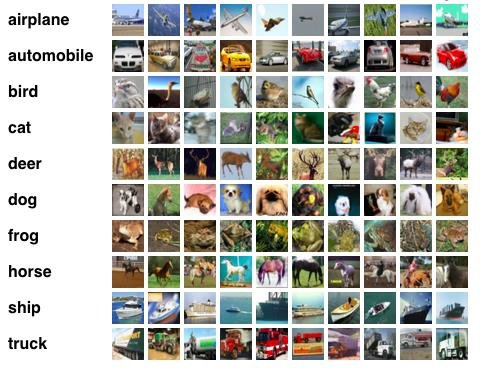
Image identification

Automated translation

Game playing

Autonomous cars (?)

Deep neural network
- Input
- Output
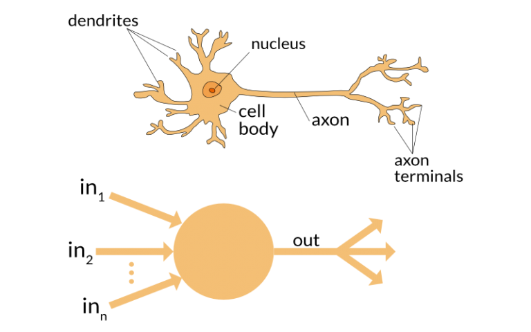
- "Neurons" where computations take place
- "Synaptic weights": model parameters
Perceptron = 1 neurônio

Perceptron (Rosenblatt'58)
\[ \sigma(x;w,a,b) = a \phi(w.x + b) \]
where \(x\in\R^d\) is the input (a vetor),
\(\phi:\R\to\R\) is a non-affine function
and \(w\in\R^d\), \(a\in\R\) , \(b\in \R\) are weights.
Perceptron (Rosenblatt'58)
\[ \sigma(x;w,a,b) = a \phi(w.x + b) \]
Common choices for \(\phi\):
- \(\phi(t) = \frac{e^t}{1+e^t}\) sigmoid
- \(\phi(t) = \max\{t,0\}\) ReLU
Training a perceptron
- Examples: pairs \((X_i,Y_i)\in\R^d\times \R,\,i=1,2,3,4,\dots\)
- Learning = adjusting \(w, a, b\) so as to minimize error.
\[\widehat{L}_n(w,a,b):=\frac{1}{n}\sum_{i=1}^n (Y_i - \sigma(X_i;w,a,b))^2.\]
Rede de 1 camada interna

Grey layer = vector of perceptrons.
\(\vec{h}=(a_i\phi(x.w_i+b_i))_{i=1}^N.\)
Output = another perceptron from gray to green
\(\widehat{y}=a\phi(w.\vec{h}+b).\)
Deep neural network (DNN)

Types of networks
- Complete connections between consecutive layers
- Convolutions (ConvNet).
- "Pooling" of small windows...
HUGE LITERATURE
How to learn weights?
- Let \(\theta\in\R^N\) be a vector containing all weights, so that the network computes: \[(x,\theta)\in\R^d\times \R^N\mapsto \widehat{y}(x;\theta).\]
- Loss: \[\widehat{L}(\theta):=\frac{1}{n}\sum_{i=1}^n(Y_i - \widehat{y}(X_i;\theta))^2.\]
- How does one try to minimize the loss?
Gradient descent
\[\theta^{(k+1)} = \theta^{(k)} - \alpha(k)\nabla\widehat{L}(\theta^{(k)})\]
"Backpropagation" (Hinton): compact form for writing gradients via chain rule.
Does it work?
Apparently yes.
\(O(10^1)\) - \(O(10^2)\) layers.
\(O(10^7)\) or more neurons per layer.
ImageNet database \(O(10^9)\) with images.
Requires a lot of computational power.
Why does it work?
Nobody knows.
This talk: some theorems towards an explanation.
Performance on CIFAR-10

Error rates down to 1% from 21%
Como formular o problema?
Statistical learning
Leo Breiman.
"Statistical Modeling: The Two Cultures" (+ discussion)
Statistical Science v. 16, issue 3 (2001).
Supervised learning
- One is given \(f:\R^d\times \Theta\to\R\).
- Goal is to choose \(\theta\in \Theta\) so as to minimize mean-squared error:
\[L(\theta):= \mathbb{E}_{(X,Y)\sim P}(Y-f(X;\theta))^2.\]
- This is "statistical" because \((X,Y)\in\R^d\times \R\) are random.
Data and empirical error
In practice, computing the exact expectation is impossible, but we have an i.i.d. sample:
\[(X_1,Y_1),(X_2,Y_2),\dots,(X_n,Y_n)\sim P.\]
Problem: how can we use the data to find a nearly optimal \(\theta\)?
Empirical error
Idea: replace expected loss by empirical loss and optimize that instead.
\[\widehat{L}_n(\theta):= \frac{1}{n}\sum_{i=1}^n(Y_i-f(X_i;\theta))^2.\]
Let \(\widehat{\theta}_n\) be the minimizer.
Why does this make sense?
Law of large numbers: for large \(n\),
\[ \frac{1}{n}\sum_{i=1}^n(Y_i-f(X_i;\theta))^2 \approx \mathbb{E}_{(X,Y)\sim P}(Y-f(X;\theta))^2 \]
\[\Rightarrow \widehat{L}_n(\theta)\approx L(\theta).\]
Mathematical theory explains the when and how: Vapnik, Chervonenkis, Devroye, Lugosi, Koltchinskii, Mendelson...
Bias and variance
Bias: if \(\Theta\) is "simple", large \(\mathbb{E}(Y-f(X;\theta))^2\) for any choice of (\theta).
Variance: if \(\Theta\) is "complex", it may be that the Law of Large Numbers does not kick in.
Underfitting & overfitting

Traditional: overfitting \(\approx\) interpolation
Small bias: check
Assume \[Y=f_*(X) + \text{noise}. \] Than some parameter setting with \(N\to +\infty\) neurons will give you a bias that is as small as you like.
Kurt Hornik (1991) "Approximation Capabilities of Multilayer Feedforward Networks", Neural Networks, 4(2), 251–257
Problems
- How do we compute the minimizer of the empirical risk?
- Is the variance actually small?
- Is a DNN uncapable of interpolation?
Gradient descent?

Erro empírico?
Teoria tradicional foi pensada para problemas convexos.
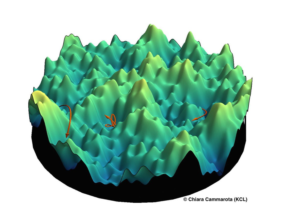
DNNs estão longe de serem convexas.
Não há garantias de que descida de gradiente converge para um mínimo global.
Mínimos locais podem ou não ser bons.
Interpolation
DNNs are capable of interpolation. Current theory is useless.
Zhang et al, "Understanding deep learning requires rethinking generalization." ICLR 2017
Min local
Teoria para métodos/estimadores que convergem para mínimos locais.
(Arora, Ge, Jordan, Ma, Loh, Wainwright, etc)
Interpolação
É possível encontrar métodos muito simples (não DNN) que interpolam e têm bons resultados em alguns casos.
(Rakhlin, Belkin, Montanari, Mei, etc)
Problema: nada disso é sobre redes neurais.
DNNs: algum progresso?
Mei, Montanari and Nguyen
Evolution of \(\mu(t)\): gradient flow in the space of probability measures over \(\R^D\).
PDEs studied by Ambrosio, Gigli, Savaré; Villani; Otto; etc.
\(\Rightarrow\) convexity in the limit.
Shallow nets are a discretization of a convex nonparametric method.
Our work
How does one extend that to deep nets.
Joint with Dyego Araújo (IMPA) e Daniel Yukimura (IMPA/NYU).
"A mean field model for certain deep neural networks"
https://arxiv.org/abs/1906.00193