Automatic Differentiation:

An Introduction

Robert Salomone

How did I get here?

I am not a computer scientist.

Application Areas

Derivative information is used in algorithms in...

Machine Learning (Optimization)
Computational Statistics (Sampling)

However...

Goals

Understand what Automatic Differentiation is and isn't.
Understand what AD is actually doing (not taking gradients!)
Demystify why Pytorch and Tensorflow are (seemingly) so weird.
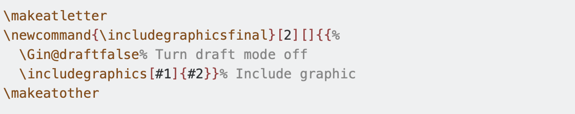
Demonstrate Autodiff in Python with some "advanced" features using Pytorch and Autograd.

The Good News

You can get (reasonably) far without knowing much.

The Not So Good News

You can get only get so far without knowing much.

The Plan

First Half: A gentle yet complete introduction to what AD is and what it is doing.

(key to understanding any AD software framework)

Second Half: Tour through two popular AD frameworks in Python, including some nice "tricks" to ease the learning curve.

Part I: Theory

Reference

Baydin et al. 2017. Automatic differentiation in machine learning: a survey. Journal of Machine Learning Research 18, 1.

What AD is not...

Finite Differences

\frac{\partial}{\partial x_i} \approx \frac{f(x_1, \ldots, x_i + h,\ldots, x_n) - f(x_1,\ldots, x_i, \ldots, x_n)}{h},

\frac{\partial f}{\partial x_i} := \lim_{h\rightarrow 0}\frac{f(x_1, \ldots, x_i + h,\ldots, x_n) - f(x_1,\ldots, x_i, \ldots, x_n)}{h}

For small $h$, we have the forward difference approximation --- $O(h)$:

\frac{\partial}{\partial x_i} \approx \frac{f(x_1, \ldots, x_i + h,\ldots, x_n) - f(x_1,\ldots, x_i-h, \ldots, x_n)}{h}.

and central difference approximation --- $O(h^2)$:

Remember what a (partial) derivative is....

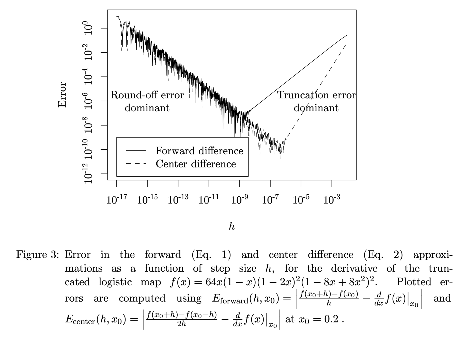
Finite differences are not only inaccurate, but also inefficient.

*from [1]

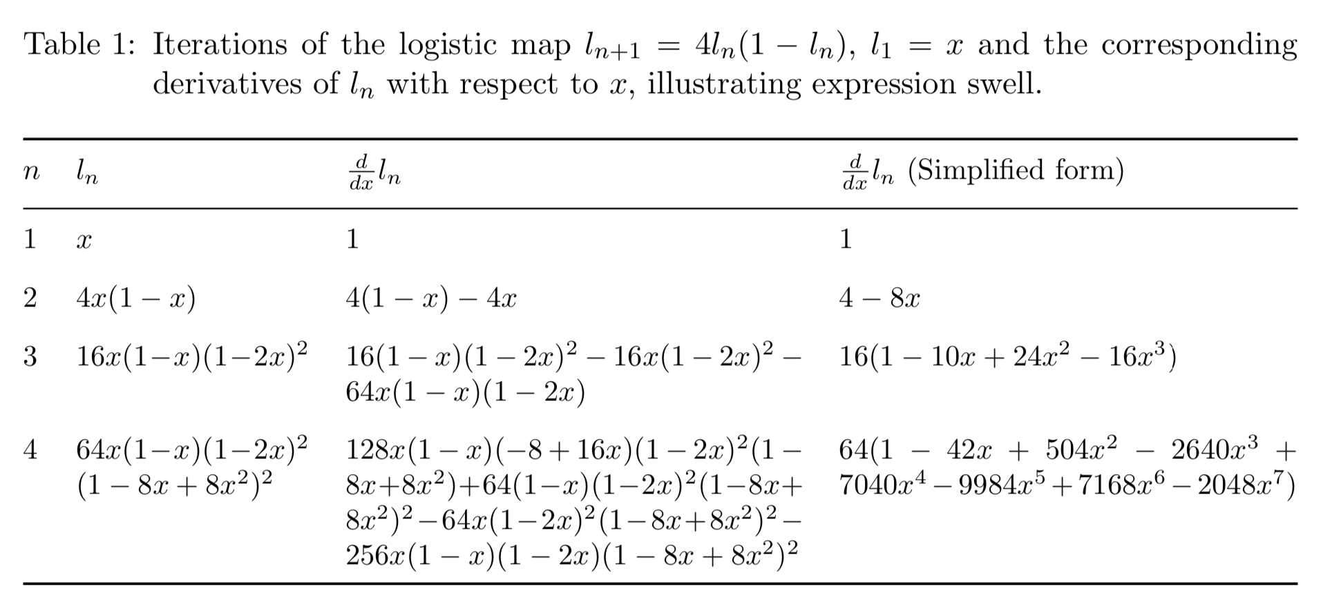
Symbolic Differentiation

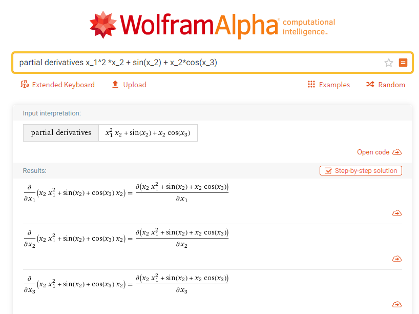
Expression Swell

* from [1]

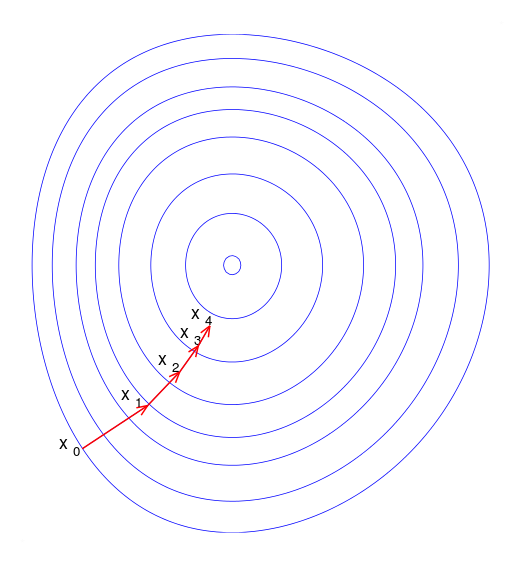
Gradients

Scalar-Valued Function $ f: \mathbb{R^n} \rightarrow \mathbb{R} $, i.e., $y = f(\mathbf{x})$.
Gradient:

\nabla f(\mathbf{x}) := \begin{pmatrix} \frac{dy}{dx_1} \\ \vdots \\ \frac{dy}{dx_n} \end{pmatrix}

Finite Difference: Approximates $\nabla f(\mathbf{x})$, requiring (at least) $n+1$ function evaluations for each desired $\mathbf{x}$.

Symbolic: Computes $\nabla f$ as its own function object. Then, requires evaluation of this object with numerical values as input.

Automatic Differentiation: Computes exactly $\nabla f(\mathbf{x})$ and $f(\mathbf{x})$. If done using the correct AD mode, it requires only (roughly) two function evaluations for each $\mathbf{x}$.

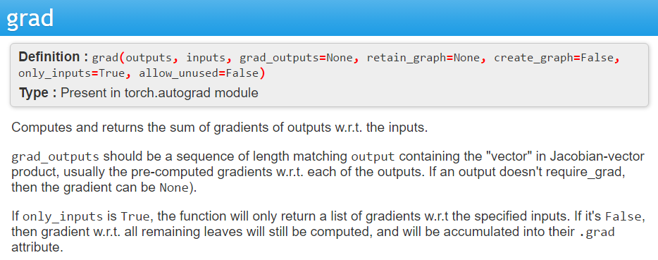
Why is PyTorch / Tensorflow so confusing?

(2) Autodiff isn't really taking partial derivatives or gradients: it is doing something else.

(1) Automatic Differentiation relies on an abstract concept called a computational graph.

Solution: Understand these concepts first, then use the software.

Computation Graphs and Primal Traces

All functions are made up of more elementary functions...

f(x_1, x_2) = z_1(x_1) + z_2(x_1,x_2) = 2x_1 + x_1 x_2

$v_3 = v_0 v_1 $

$x_1$

$v_4 = v_2 + v_3$

$x_2$

$v_2 = 2 v_0 $

$v_0$

$v_1$

Primal Trace

Computation Graph for $f(x_1, x_2) = 2x_1 + x_1 x_2 $

$f$

$y$

v_0 = x_1 \\ v_1 = x_2 \\ v_2 = 2v_0 \\ v_3 = v_0 v_1 \\ v_4 = v_2 + v_3

Exercise 1 (Graphs and Primal Trace)

Draw the computation graph and list the primal trace for the function

$f(x_1, x_2) = \log(x_1) + x_1 x_2 - \sin(x_2)$

Note: The graph and primal trace in general are not unique (different order / labels).

Hint: Pretend you are actually evaluating the function, and keep a running journal of what you do.

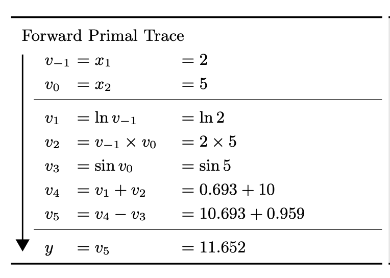
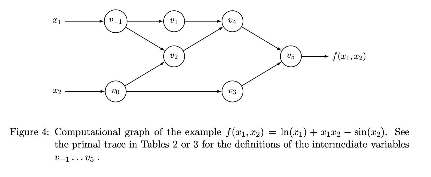
Solution (from Reference)

A graph is all you need...

Autodiff only requires a computational graph for the input of interest.
Can include recursions, conditionals (if statements), loops, etc.
- When you run the function, it just needs to take a trace of what it does with that input!
This can include "fancy" stuff like...
- ODE Solver (Runge-Kutta, Implicit Euler)
- Fast Fourier Transform
- Matrix Cholesky Factorization
- Matrix (log-)Determinant

Reminder: Multivariate Chain Rule

$z_2(x_1, x_2) = x_1 x_2 $

\frac{\partial y}{\partial x_1}=

\frac{\partial y}{\partial z_1}\frac{\partial z_1}{\partial x_1}

+\frac{\partial y}{\partial z_2}\frac{\partial z_2}{\partial x_1}

$x_1$

$y(z_1(x_1), z_2(x_1, x_2))$

$\qquad= 2x_1 + z_2(x_1, x_2)$

$x_2$

$z_1(x_1) = 2 x_1 $

f(x_1, x_2) = z_1(x_1) + z_2(x_1,x_2) = 2x_1 + x_1 x_2

Multivariate Chain Rule

$z_2(x_1, x_2) = x_1 x_2 $

\frac{\partial y}{\partial x_2}=

\frac{\partial y}{\partial z_2}\frac{\partial z_2}{\partial x_2}

$x_1$

$y(z_1(x_1), z_2(x_1, x_2))$

$\qquad= 2x_1 + z_2(x_1, x_2)$

$x_2$

$z_1(x_1) = 2 x_1 $

f(x_1, x_2) = z_1(x_1) + z_2(x_1,x_2) = 2x_1 + x_1 x_2

Forward (Tangent) Mode AD

\dot{v}

$v_3 = v_0 v_1 $

$x_1$

$v_4 = v_2 + v_3$

$x_2$

$v_2 = 2 v_0 $

$v_0$

$v_1$

$f$

$y$

f(x_1, x_2) = z_1(x_1) + z_2(x_1,x_2) = 2x_1 + x_1 x_2

Primal Trace

v_0 = x_1 \\ v_1 = x_2 \\ v_2 = 2v_0 \\ v_3 = v_0 v_1 \\ v_4 = v_2 + v_3

(Partial) Tangent Trace

$$\dot{v}_{k,i} := \frac{\partial v_k}{\partial x_{i}}$$

$v_3 = v_0 v_1 $

$x_1$

$v_4 = v_2 + v_3$

$x_2$

$v_2 = 2 v_0 $

$v_0$

$v_1$

$f$

$y$

(Partial) Tangent Trace: $\dot{v}_{k,i} := \frac{\partial v_k}{\partial x_{i}}$

$\dot{v}_{0,1} = \frac{\partial v_0}{\partial x_1}=1$

$\dot{v}_{2,1} = \frac{\partial v_2}{\partial x_1}=\frac{\partial v_2}{\partial v_0}\frac{\partial v_0}{\partial x_1}= \frac{\partial v_2}{\partial v_0}\dot{v}_{0,1} $

$\dot{v}_{3,1} = \frac{\partial v_3}{\partial x_1}=\frac{\partial v_3}{\partial v_0}\frac{\partial v_0}{\partial x_1}= \frac{\partial v_3}{\partial v_0}\dot{v}_{0,1} $

$\dot{v}_{4,1} = \frac{\partial v_4}{\partial x_1}=\frac{\partial v_4}{\partial v_2}\frac{\partial v_2}{\partial x_1} + \frac{\partial v_4}{\partial v_3}\frac{\partial v_3}{\partial x_1}= \frac{\partial v_4}{\partial v_3}\dot{v}_{2,1} + \frac{\partial v_4}{\partial v_3}\dot{v}_{3,1} $

Key Aspect: only expand the chain rule once at each stage, reusing the (forward) accumulated derivatives.

Intuition

Primal Trace

v_0 = x_1 \\ v_1 = x_2 \\ v_2 = 2v_0 \\ v_3 = v_0 v_1 \\ v_4 = v_2 + v_3

f(x_1, x_2) = z_1(x_1) + z_2(x_1,x_2) = 2x_1 + x_1 x_2

Differentiability

In practice, we only need the function to be differentiable at the points we evaluate it along the tangent trace.

So e.g., the absolute value function $|\cdot |$

is not problematic in practice so long as we don't input zero!

Let's generalize a little...

\dot{v}_k := \sum_{v_i \in {\rm parents}(v_k)}\frac{\partial v_k}{\partial v_i}\dot{v}_i.

The above is are elements of what is called the tangent trace.

Note: Initializing $\dot{\mathbf{x}} = (1,0)$ or $\dot{\mathbf{x}}=(0,1) $ makes $\dot{y}$ be the derivative with respect to $x_1$ or $x_2$ respectively.

Let's now consider

$v_3 = v_0 v_1 $

$x_1$

$v_4 = v_2 + v_3$

$x_2$

$v_2 = 2 v_0 $

$v_0$

$v_1$

$f$

$y$

$\dot{v}_0 = \dot{x}_1$

$\dot{v}_1 = \dot{x}_2$

$\dot{v}_3 = \dot{v}_0 v_1 + v_0 \dot{v}_1$

$\dot{v}_2 = 2\dot{v}_0 $

$\dot{v}_4 = \dot{v}_2 + \dot{v}_3 $

$\dot{y}$

\dot{v}_k := \sum_{v_i \in {\rm parents}(v_k)}\frac{\partial v_k}{\partial v_i}\dot{v}_i

Exercise 2 (Forward Mode)

\dot{v}_k := \sum_{i \in {\rm parents}(v_k)}\frac{\partial v_k}{\partial v_i}\dot{v}_i

With the function from the last example, compute the tangent trace for each graph node.

$f(x_1, x_2) = \log(x_1) + x_1 x_2 - \sin(x_2)$

Then, use it to evaluate $\frac{\partial f}{\partial x_1} $ at (2,5) by setting $\dot \mathbf{x} = (1,0) $

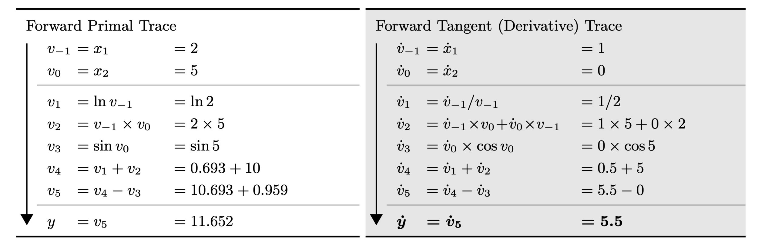
Solution

...doesn't that add redundant computation?

No, it adds magic.

(click above for answer)

Name that Mathematician

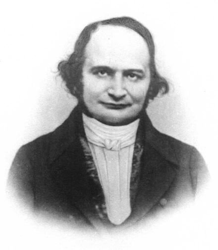
Carl Gustav Jacob Jacobi

Most famous for:

theory of elliptic functions

(also that matrix of derivatives from second-year calculus)

Jacobian Matrix

\mathrm{J}_{\mathbf{f}} := \begin{bmatrix} \frac{dy_1}{dx_1} & \cdots & \frac{dy_1}{dx_n} \\ \vdots& \ddots& \vdots \\ \frac{dy_m}{dx_1} & \cdots & \frac{dy_m}{dx_n} \\ \end{bmatrix}

Quiz: The $k $-th row of $ \mathrm{J}_{\mathbf{f}}(\mathbf{x}) $ is equal to

\nabla y_k(\mathbf{x})

\mathbf{f}(\mathbf{x}) = (f_1(\mathbf{x}), \ldots, f_m(\mathbf{x})) = \mathbf{y}

$\mathbf{f}: \mathbb{R}^n \rightarrow \mathbb{R}^m $

\mathrm{J}_{\mathbf{f}} \in \mathbb{R}^{m \times n}

Jacobian-Vector Product (JVP)

\mathrm{J}_{\mathbf{f}}(\mathbf{x})\, \dot{\mathbf{x}} = \begin{bmatrix} \frac{dy_1(\mathbf{x})}{dx_1} & \cdots & \frac{dy_1(\mathbf{x})}{dx_n} \\ \vdots& \ddots& \vdots \\ \frac{dy_m(\mathbf{x})}{dx_1} & \cdots & \frac{dy_m(\mathbf{x})}{dx_n} \\ \end{bmatrix} \begin{bmatrix} \dot{x}_1 \\ \vdots \\ \dot{x}_n \end{bmatrix} =\begin{bmatrix} s_1 \\ \vdots \\ s_m \end{bmatrix}

Forward Mode actually evaluates this for arbitrary $\dot{\mathbf{x}}$.

The Jacobian of a scalar-valued function $f: \mathbb{R}^n \rightarrow \mathbb{R} $ is its ...

gradient transposed: $\nabla f(\cdot)^\top$.

In this case, the Jacobian-Vector product is equal to

\nabla f(\mathbf{x})^\top \mathbf{\dot{x}} = s,

i.e., the

Directional Derivative of $f$($\mathbf{x} $) in the direction $\mathbf{\dot{x}}$.

Look at one part...

$v_3 = v_0 v_1 $

$x_1$

$x_2$

$v_2 = 2 v_0 $

$v_0$

$v_1$

$\dot{v}_0 = \dot{x}_1$

$\dot{v}_1 = \dot{x}_2$

$\dot{v}_3 = \dot{v}_0 v_1 + v_0 \dot{v}_1$

$\dot{v}_2 = 2\dot{v}_0 $

\mathrm{J}_{v_3} = \big[\frac{\partial v_3}{\partial v_0}, \frac{\partial v_3}{\partial v_1}\big] = \big[ v_0, v_1\big]

\dot{v_3} = \mathrm{J}_{v_3}\begin{pmatrix} \dot{v}_0 \\ \dot{v}_1 \end{pmatrix}

So...

\dot{v}_k := \sum_{i \in {\rm parents}(v_k)}\frac{\partial v_k}{\partial v_i}\dot{v}_i = \mathrm{J}_{v_k}\dot{v}_{{\rm parents}(v_k)}

Forward accumulation computes JVPs and passes them forward...

Note that we never need to form the full Jacobian matrix/matrices!

The "Magic"

We can initialize $\dot{\mathbf{x}} = \mathbf{r}$ and compute any JVP: $\mathrm{J}_f(\mathbf{x}) \mathbf{r} $ in only one pass through the computation graph!

For $f: \mathbb{R}^n \rightarrow \mathbb{R}$, initializing with $\dot{\mathbf{x}}=\mathbf{e}_i$ gives the $i$-th partial derivative.

This involves roughly the same effort as computing the initial function twice!

More generally...

\mathrm{J}_{\mathbf{f}}(\mathbf{x}) \begin{bmatrix} 0 \\ \vdots \\ 1 \end{bmatrix} = \begin{bmatrix} \frac{dy_1}{dx_1} & \cdots & \frac{dy_1}{dx_n} \\ \vdots& \ddots& \vdots \\ \frac{dy_m}{dx_1} & \cdots & \frac{dy_m}{dx_n} \\ \end{bmatrix} \begin{bmatrix} 0 \\ \vdots \\ 1 \end{bmatrix} =

\mathbf{f}(\mathbf{x}) = (f_1(\mathbf{x}), \ldots, f_m(\mathbf{x})) = \mathbf{y}

$\mathbf{f}: \mathbb{R}^n \rightarrow \mathbb{R}^m $

One forward mode sweep can evaluate a column of the Jacobian at $\mathbf{x}$!

Setting $\dot{\mathbf{x}} = \mathbf{e}_i$ evaluates the $i$-th column.

\begin{bmatrix} \frac{dy_1}{dx_m} \\ \vdots \\ \frac{dy_m}{dx_n} \\ \end{bmatrix}

Quiz

Forward mode requires sweeps of the graph to evaluate the full Jacobian.

For $m=1$, $\nabla f(\mathbf{x}) = \mathrm{J}_f (\bf x)^\top $ :(

\mathbf{f}: \mathbb{R}^n \rightarrow \mathbb{R}^m,\quad \mathrm{J}_{\mathbf{f}} \in \mathbb{R}^{m \times n} \text{ (Jacobian)}

For $n=1, \mathrm{J}_f(\mathbf{x}) = \mathrm{J}_{f}(\mathbf{x})\times 1$ :D

Reverse (Adjoint) Mode AD

\overline{v}

Back to Multivariate Chain Rule

$z_2(x_1, x_2) = x_1 x_2 $

\frac{\partial y}{\partial x_1}=

\frac{\partial y}{\partial z_1}\frac{\partial z_1}{\partial x_1}

+\frac{\partial y}{\partial z_2}\frac{\partial z_2}{\partial x_1}

$x_1$

$y(z_1(x_1), z_2(x_1, x_2))$

$\qquad= 2x_1 + z_2(x_1, x_2)$

$x_2$

$z_1(x_1) = 2 x_1 $

f(x_1, x_2) = z_1(x_1) + z_2(x_1,x_2) = 2x_1 + x_1 x_2

Reverse Mode is Generalized Backpropagation

\widehat{y} = {\rm W}_2 \, {\rm max}\left\{\mathbf{0},{\rm W}_1 \mathbf{x} + b_1\right\} + b_2

\text{Loss}(\widehat{y},y)

$\widehat{y}$

$y$

$b_1$

$b_2$

$x_1$

$x_2$

$x_3$

Neural Net Loss Function: Backpropagation

Everything Else:

Reverse Mode AD

(Partial) Adjoints

\overline{v}_{k,i} = \frac{\partial y_i}{\partial v_k}

compare with (Partial) Tangents:

\dot{v}_{k,i} := \frac{\partial v_k}{\partial x_i}

\overline{v}_k := \sum_{i \in {\rm children}(v_k)}\textcolor{blue}{\frac{\partial v_i}{\partial v_k}}\overline{v}_i

\dot{v}_k := \sum_{i \in {\rm parents}(v_k)}\textcolor{red}{\frac{\partial v_k}{\partial v_i}}\dot{v}_i

(tangents go) Forward Accumulation

(adjoints go) Backward Accumulation

\overline{v}

\dot{v}

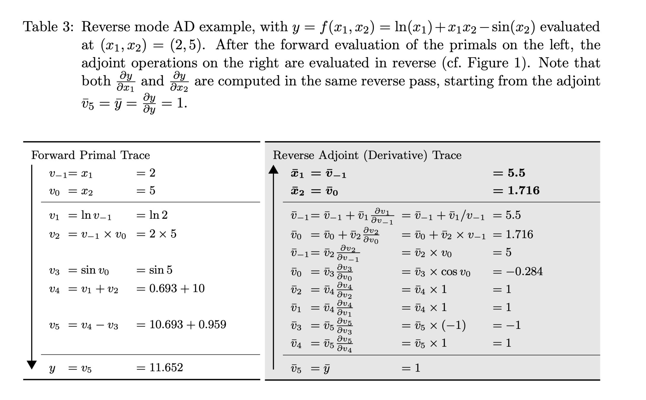
Exercise 3 (Reverse Mode)

\dot{v}_k := \sum_{i \in {\rm parents}(v_k)}\frac{\partial v_k}{\partial v_i}\dot{v}_i

With the function from the last exercises, compute the adjoint trace for each graph node.

$f(x_1, x_2) = \log(x_1) + x_1 x_2 - \sin(x_2)$

Solution

Vector Jacobian Product (VJP)

(\mathbf{r}^\top \mathrm{J}_f)^\top = \mathrm{J}_f^\top \mathbf{r} = \begin{bmatrix} \frac{dy_1}{dx_1} & \cdots & \frac{dy_1}{dx_n} \\ \vdots& \ddots& \vdots \\ \frac{dy_m}{dx_1} & \cdots & \frac{dy_m}{dx_n} \\ \end{bmatrix}^\top \begin{bmatrix} r_1 \\ \vdots \\ r_m \end{bmatrix} =\begin{bmatrix} s_1 \\ \vdots \\ s_n \end{bmatrix}^\top

Evaluate the VJP by initializing the reverse phase with $$ \overline{\mathbf{y}} = \mathbf{r}.$$

\overline{v}_k := \sum_{i \in {\rm children}(v_k)}\textcolor{blue}{\frac{\partial v_i}{\partial v_k}}\overline{v}_i

Key Observation

This single node "backpropagation" is a Vector-Jacobian product!

$v_3 = v_0 v_1 $

$x_1$

$x_2$

$v_2 = 2 v_0 $

$v_0$

$v_1$

$\overline{v}_0$

$\overline{v}_1 = \overline{x}_2$

$\overline{v}_3 $

$\overline{v}_2 $

$v_3 = {\rm SOLVE}_{\mathbf{y}} (\mathrm{v_0}\mathbf{y}=v_1)$

$\mathrm{A}$

$v_4 = v_2 v_3$

$\mathbf{x}$

$v_2 = \mathrm{A}^{1/2}$

$v_0$

$v_1$

Graph nodes need not contain elementary operations: you can compress it so long as you know a nodes VJP function!

$f$

$\mathbf{y}$

Primatives

Recall that Forward Mode with unit vectors for $\dot{\mathbf{x}}$ evaluates a column of the Jacobian.

Backward Mode with unit vectors for $\dot{\mathbf{x}}$ evaluates a row of the Jacobian.

So what's it do?

Quiz (Reverse Mode)

For $f: \mathbb{R}^n \rightarrow \mathbb{R}$, we can evaluate the gradient with backward sweep(s).

For $f: \mathbb{R} \rightarrow \mathbb{R}^m$, we can obtain the Jacobian with backward sweep(s).

$\nabla(\mathbf{x})^\top = 1 \times {\rm J_f}(\mathbf{x}) $

(one row each time)

Automatic Differentiation: Summary

AD Mode	Operation
Forward	JVP:	Column
Backward	VJP:	Row

\mathbb{R}^n \rightarrow \mathbb{R}^m

\mathbb{R}^m \rightarrow \mathbb{R}^n

\mathrm{J}_{\mathbf{f}}[i,:](\mathbf{x})

\mathrm{J}_{\mathbf{f}}[:,i](\mathbf{x})

(\dot{\mathbf{x}} \in \mathbb{R}^n)

(\overline{\mathbf{y}} \in \mathbb{R}^m)

\dot{\mathbf{x}}/\overline{\mathbf{y}} = \mathbf{e}_i

\mathbf{f}: \mathbb{R}^n \rightarrow \mathbb{R}^m,\quad \mathrm{J}_{\mathbf{f}} \in \mathbb{R}^{m \times n} \text{ (Jacobian)}

\big(\nabla f(\mathbf{x})^\top \text{ for } m=1\big)

\overline{\mathbf{y}}^\top \mathrm{J}_{\mathbf{f}} = (\mathrm{J}_{\mathbf{f}}^\top \overline{\mathbf{y}})^\top

\mathrm{J}_{\mathbf{f}}\dot{\mathbf{x}}

Can you combine the two in smart ways?

Yes

(I'll give you the most useful example...)

Hessians

\mathrm{H}_f(\mathbf{x}) := \begin{bmatrix} \frac{dy}{\partial x_1 \partial x_1} & \cdots & \frac{dy}{\partial x_1 \partial x_n} \\ \vdots& \ddots& \vdots \\ \frac{dy}{\partial x_n \partial x_1} & \cdots & \frac{dy_m}{dx_n dx_n} \\ \end{bmatrix}

Suppose that $ f: \mathbb{R}^n \rightarrow \mathbb{R} $. Then, the Hessian of $f $ is

$${\rm H}_{f}(\mathbf{x}) = \mathrm{J_{\nabla f}}(\mathbf{x}) = \textcolor{red}{\nabla} \big( \nabla f(\mathbf{x})\big)$$

The Hessian is the of the of $f$

gradient

Jacobian

VJP (Forward Mode) to obtain trace of (*) $\mathbf{u}^\top\nabla f(\mathbf{x}) $
Take Gradient of (*) (Reverse Mode):

\nabla\left(\mathbf{r}^\top \nabla f(\mathbf{x})\right) = \mathbf{r}^\top \nabla\nabla f(\mathbf{x}) = \mathbf{r}^\top {\rm H} = ({\rm H}\mathbf{r})^\top

Hessian Vector Product (HVP)

Requires effort of (roughly) only four function evaluations!

Inverse-Hessian Vector Product

Can even evaluate $\mathrm{H}^{-1}\mathbf{r}$ by touching only HVPs (using the Conjugate Gradient method).

e.g., Neural Net with with $10^6$ parameters. Hessian has $10^{12}$ elements: 8 terabytes!

Question and Discussion Time!

Part II : Practice

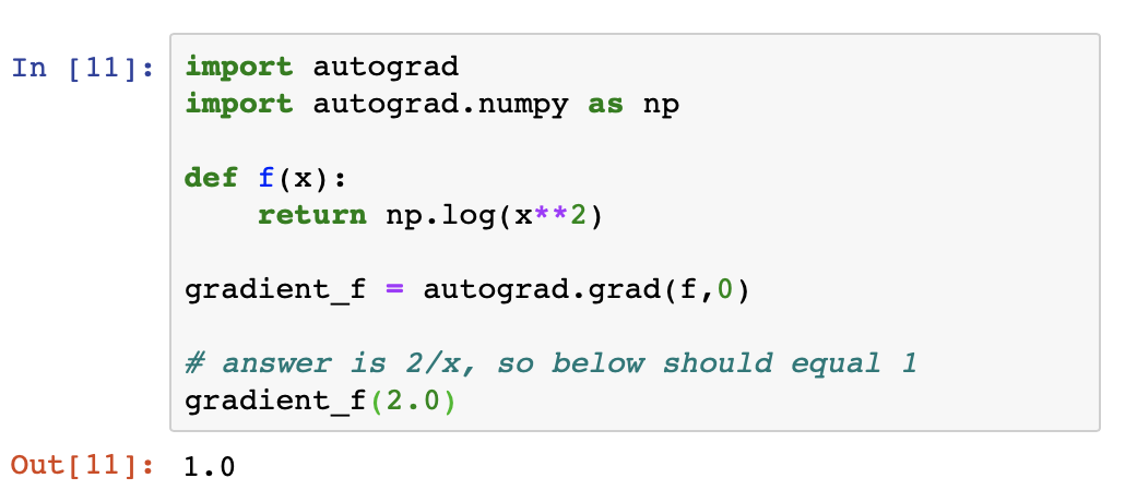
With its updated version of Autograd, JAX can automatically differentiate native Python and NumPy functions.

Graphics Processing Units (GPUs)

Good at doing many linear algebra operations (VJP/JVP) at once.

$v_3 = {\rm SOLVE}_{\mathbf{y}} (\mathrm{v_0}\mathbf{y}=v_1)$

$\mathrm{A}$

$v_4 = v_2 v_3$

$\mathbf{x}$

$v_2 = \mathrm{A}^{1/2}$

$v_0$

$v_1$

$f$

$\mathbf{y}$

$\overline{v}_1$:JVP-2

$ \overline{v}_0$:JVP-1

Parallelization

	Forward Mode	Reverse Mode	GPU
Tensorflow
PyTorch
Autograd
Jax (Autograd 2.0)

\checkmark

\text{\sf X}

Python Frameworks

Generally reverse mode will be enough, but beware!

Where's the VJP?!

See A New Trick for Calculating Jacobian Vector Products

Using software that doesn't have forward mode?

You can get a JVP using a VJP of a VJP.

See Jupyter Notebook for the rest!

Automatic Differentiation:

An Introduction

How did I get here?

Application Areas

However...

Goals

The Good News

The Not So Good News

The Plan

Part I: Theory

Reference

What AD is not...

Finite Differences

Symbolic Differentiation

Expression Swell

Gradients

Why is PyTorch / Tensorflow so confusing?

Computation Graphs and Primal Traces

All functions are made up of more elementary functions...

Computation Graph for \(f(x_1, x_2) = 2x_1 + x_1 x_2 \)

Exercise 1 (Graphs and Primal Trace)

A graph is all you need...

Reminder: Multivariate Chain Rule

Multivariate Chain Rule

Forward (Tangent) Mode AD

(Partial) Tangent Trace

$$\dot{v}_{k,i} := \frac{\partial v_k}{\partial x_{i}}$$

Intuition

Let's generalize a little...

Exercise 2 (Forward Mode)

Solution

...doesn't that add redundant computation?

Name that Mathematician

Jacobian Matrix

Jacobian-Vector Product (JVP)

Look at one part...

So...

The "Magic"

More generally...

Quiz

Reverse (Adjoint) Mode AD

Back to Multivariate Chain Rule

Reverse Mode is Generalized Backpropagation

Neural Net Loss Function: Backpropagation

Everything Else:

Reverse Mode AD

(Partial) Adjoints

(tangents go) Forward Accumulation

(adjoints go) Backward Accumulation

Exercise 3 (Reverse Mode)

Solution

Vector Jacobian Product (VJP)

Key Observation

Primatives

So what's it do?

Quiz (Reverse Mode)

Automatic Differentiation: Summary

Can you combine the two in smart ways?

Hessians

Part II : Practice

Graphics Processing Units (GPUs)

Python Frameworks

Where's the VJP?!

See Jupyter Notebook for the rest!