Convex Learning
Outline
- Convex Learning Problem
- Useful Properties
- Learnability
- Surrogate Loss Function
- Regularization and Stability
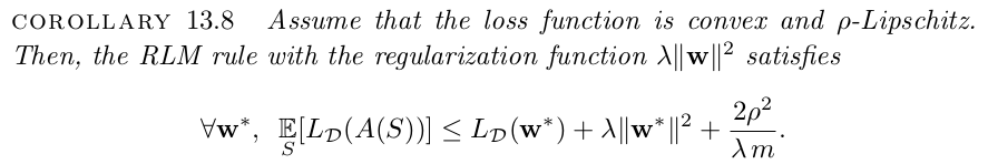
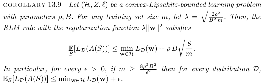
- Regularized Loss Minimization
- Fitting-Stability Tradeoff
- Stochastic Gradient Descent
- Learning with SGD
In fact, we know it
- Linear regression with square loss
- Logistic regression
Convex set
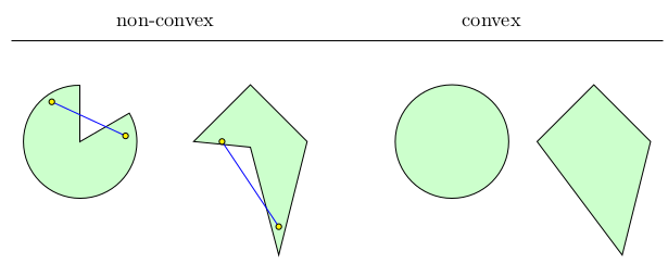
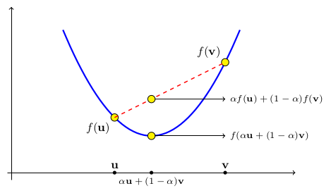
Convex function
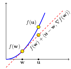
First Order Property
Second order Property
For function f with f' and f'' exists, TFAE
- f is convex
- f' is monotonically increasing
- f'' is nonegative
Examples
Linear transformation preserves convexity
is convex when
is convex
is convex and so is
is convex
Obviously,
Other functions preserve convexity
Logistic loss is convex
Proofs
Lipschitzness
Lipschitzness
For a differentiable function f, it is -lipschitz if and only if
in 1-D case
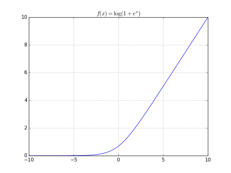
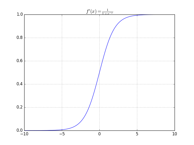
is 1-Lipschitz
Bounded by [-1, 1]
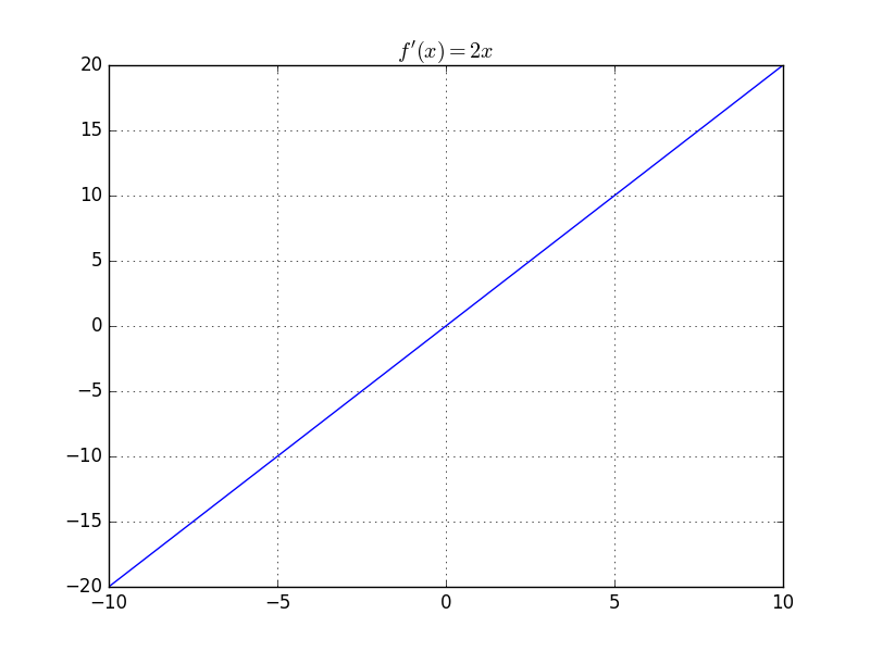
is not Lipschitz
Unbounded above!
Smoothness
A function is called -smooth when its derivative is -lipschitz
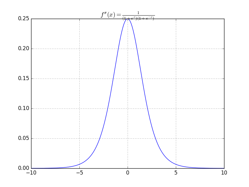
is 1/4-smooth
Bounded by [-1/4, 1/4]
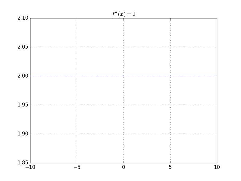
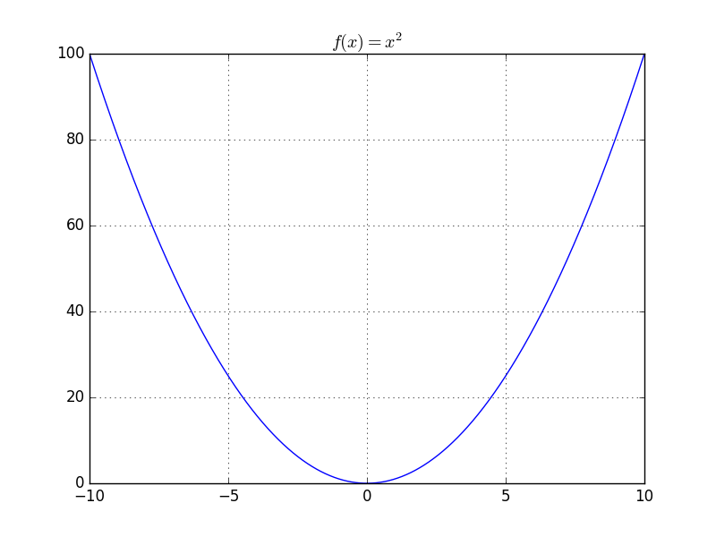
is 2-smooth
bounded by [-2,2]
Property of smoothness
Self-bounded
When f is non-negative and smooth we can obtain
by setting
in
Lipschitzness and smoothness under linear transformation
is -lipschitz then
is -lipschitz
is -smooth then
is -smooth
Examples
-lipschitz and -smooth
Since
Examples
-smooth
Boundness of training set
In previous arguement, we have the form like -smooth
But x is a variable, so we also need x to be bounded :
So that we can say a loss function is -smooth
Proofs
Convex learning problem
A learning problem with
- convex set H
- loss function convex in h
So linear regression and logistic regression are convex learning problems
Convex learning problem and convex optimization problem
When we apply ERM rule to a convex learning problem, we are finding the minimum of convex function
which is equivalent to solving a convex optimization problem
Learnability of convex learning problems
Two kinds of convex learning problems are learnable :
- Convex-Lipschitz-Bounded problem
- Convex-Smooth-Bounded problem
Convex learning problem is not learnable in general
Example 12.8
Example 12.8
Example 12.9
Example 12.9
Surrogate Loss Function
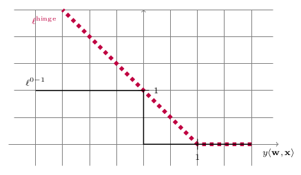
Surrogate Loss Function
Regularization and Stability
- Regularized Loss Minimization
- Stability and Overfitting
- Proof of Learnability
- Convex-Lipschitz-Bounded problem
- Convex-Smooth-Bounded problem
RLM learning rule
Tikhonov Regularization
Ridge Regression
Stability
Stability and Overfitting
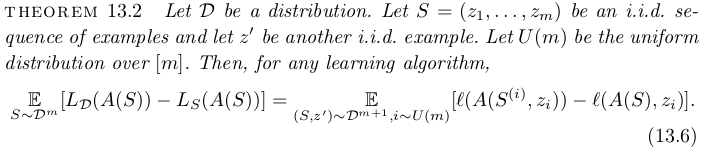
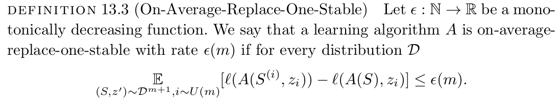
Replace-One-Stable
Strong Convex
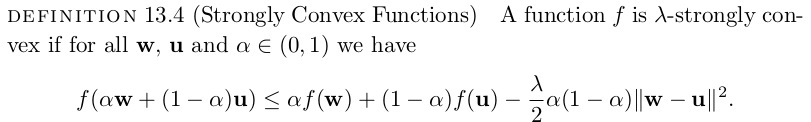
Strong Convex

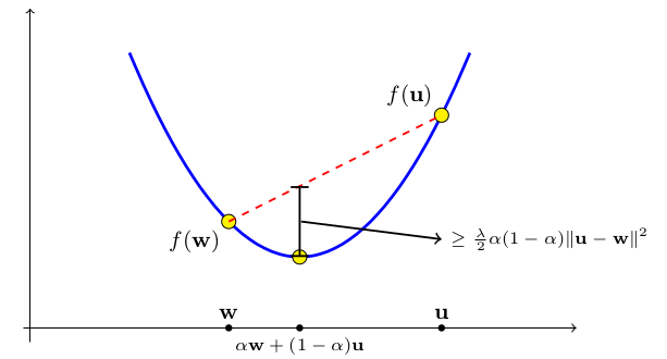
Strong convex
Replace-One-Stable
Author abuse the fact that the loss function is strong convex in this proof
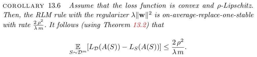
RLM Stability-Fitting Tradeoff


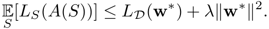

Lipschitzness would help
Stochastic Gradient Descent
- Gradient Descent to SGD
- Learning with SGD
- Comparison of SGD and RLM
- Appliction of SGD
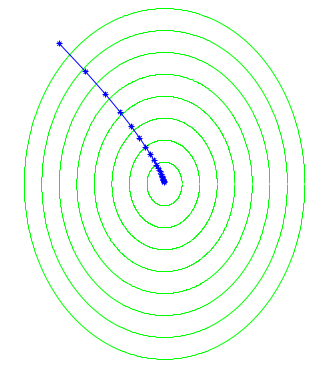
Gradient Descent
Importance of Lipschitzness and Smoothness
Lipschitzness
Self-bounded(Smoothness)
Gradient Descent
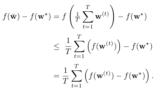
Gradient Descent
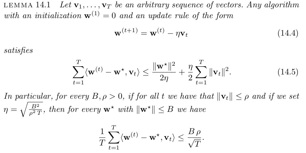
Stochastic Gradient Descent
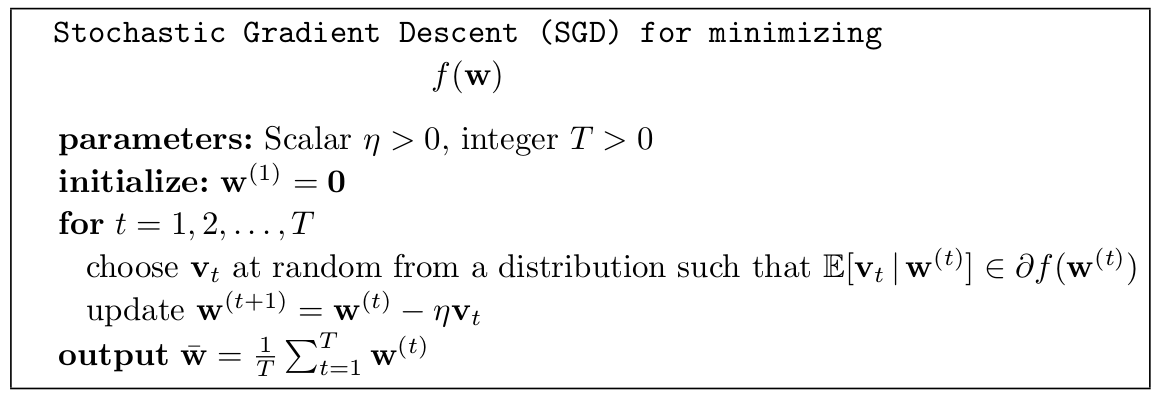
Stochastic Gradient Descent
same as GD
What if we go out of boundary?
What if we have strong convexity?
SGD Learning
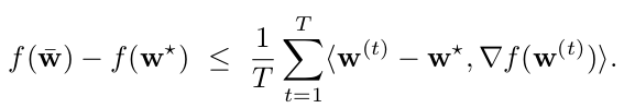
We directly minimize the true risk with an unbiased estimate of its gradient

Followed by SGD method we can obtain the result we want
Comparison
convex-Lipschitz-bounded
convex-Smooth-bounded
| samples / Iterations | RLM | SGD |
|---|---|---|
|
|
||
|
|
Learning
Rule
Specific
Algorithm
Application
When training DNN, SGD is the most common algorithm to train the NN model
- Hypothesis set is all possible neural network
- Implement SGD by batches of training data
- ERM rule apply to choose best DNN model
- Usually use square loss function
- In general, the loss function is not convex
SGD with Momentum
In practice SGD is a successful method in training DNN
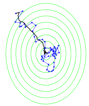
- SGD itself will introduce randomness
- SGD with momentum will avoid local minimum
- Local minimum is few in practical problem
Other Issue of SGD
- Properly selection of initial position
- Boosting the efficiency : RMSProp, adagrad
- Proper batch size selection
- Back propagation to evaluate gradient