Constraining modifications of gravity with synergies between radio and optical surveys
Santiago Casas,
with Isabella Carucci, Valeria Pettorino,
Stefano Camera, Matteo Martinelli

arXiv:2210.05705 Phys.Dark Univ. 39 (2023) 101151
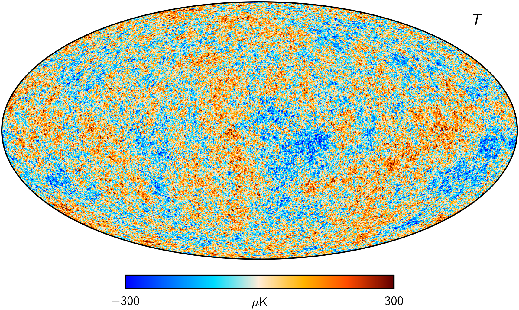
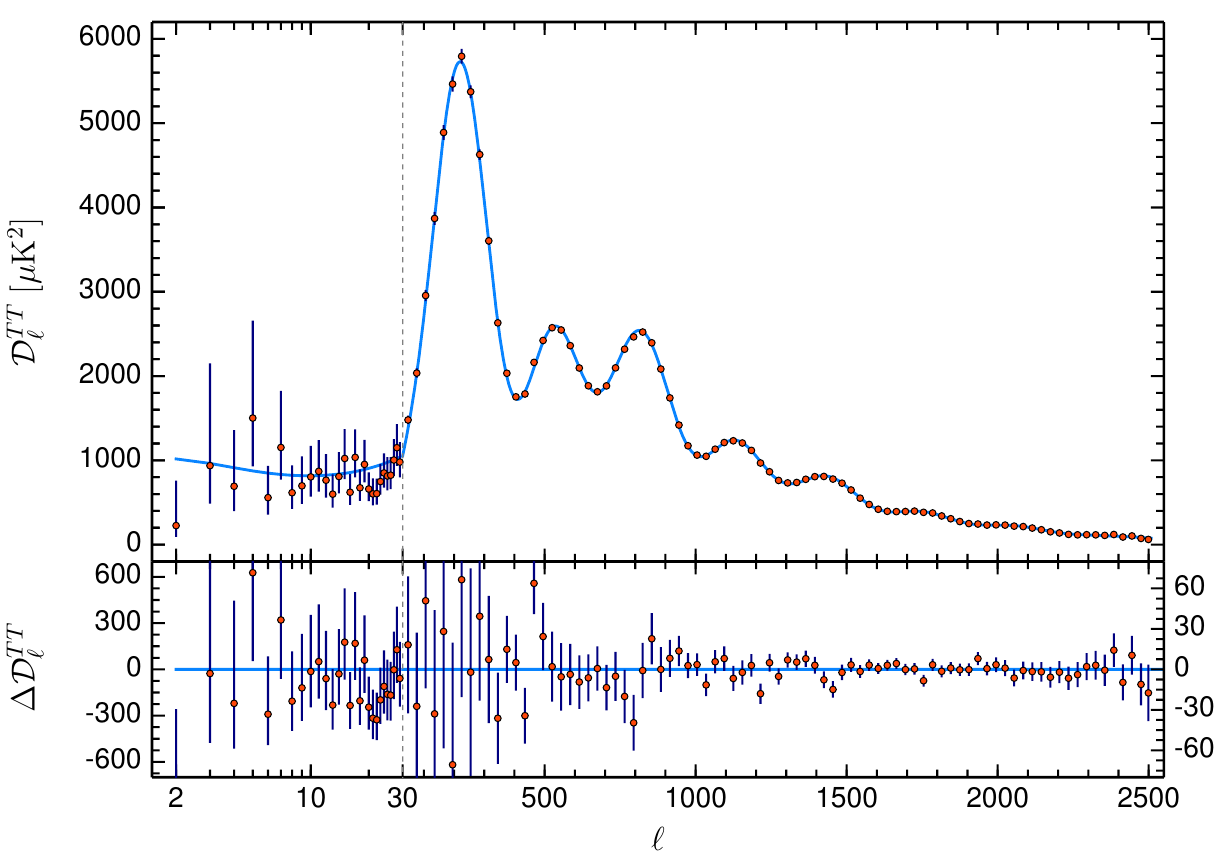
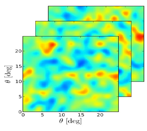
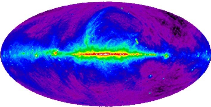
Cosmic Microwave Background
Planck 2018 CMB Temperature map (Commander) . wiki.cosmos.esa.int/planck-legacy-archive/index.php/CMB_maps
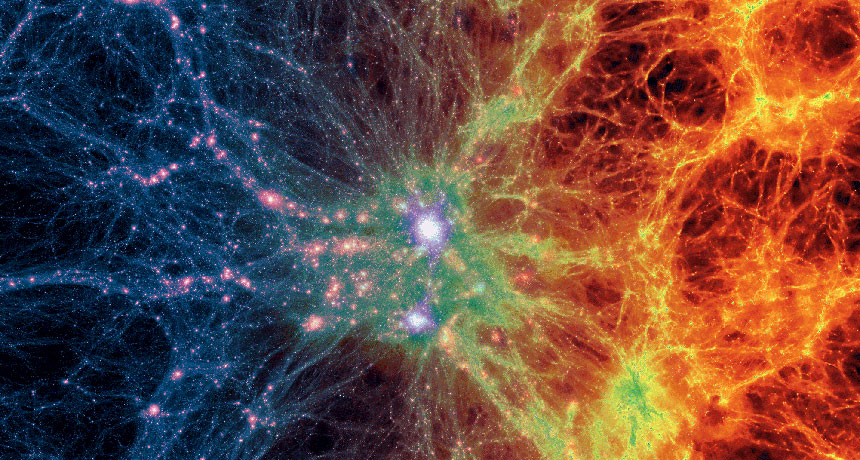
Large Scale Structure
Illustris Simulation: www.nature.com/articles/nature13316
Santiago Casas, 17.01.23
The Standard \(\Lambda\)CDM model
- \(\Lambda\)CDM is still best fit to observations.
- Predictive model with few free parameters.
- Lensing
- CMB
- Clustering
- Supernovae
- Clusters
Concordance Cosmology:
Santiago Casas, 17.01.23
The Standard \(\Lambda\)CDM model
- \(\Lambda\)CDM is still best fit to observations.
- Some questions remain:
- \(\Lambda\) and CDM.
- Cosmological Constant Problem:
O(100) orders of magnitude wrong
(Zeldovich 1967, Weinberg 1989, Martin 2012).
Composed of naturalness and coincidence
sub-problems, among others.
Quantum Gravity?
Santiago Casas, 17.01.23
Tensions in the \(\Lambda\)CDM model
- \(\Lambda\)CDM is still best fit to observations.
- Some questions remain:
- H0 tension, now ~5\(\sigma\)

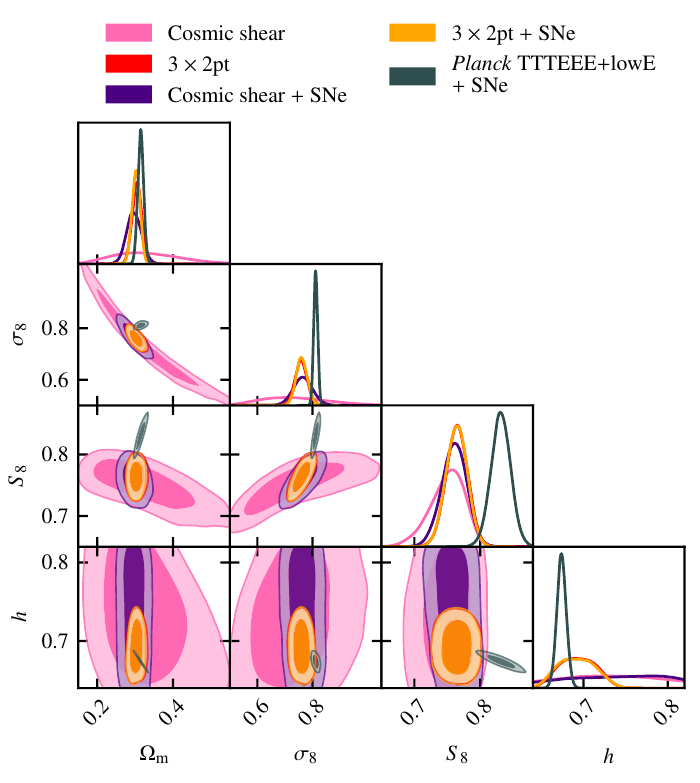
Planck, Clusters and Lensing tension on clustering amplitude \(\sigma_8\)
KiDS 1000 Cosmology, arXiv:2010:16416
L.Verde, et al 2019. arXiv:1907.10625
Santiago Casas, 17.01.23
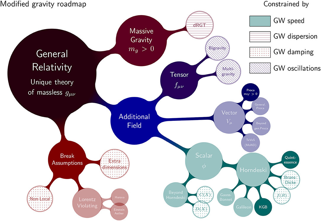
Alternatives to \(\Lambda\)CDM
Ezquiaga, Zumalacárregui, Front. Astron. Space Sci., 2018
Santiago Casas, 17.01.23
Parametrized modified gravity

In \(\Lambda\)CDM the two linear gravitational potentials \(\Psi\) and \(\Phi\) are equal to each other
We can describe general modifications of gravity (of the metric) at the linear level with 2 functions of scale (\(k\)) and time (\(a\))
Only two independent functions
Santiago Casas, 17.01.23
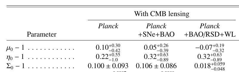
Late-time parametrization: Planck constraints
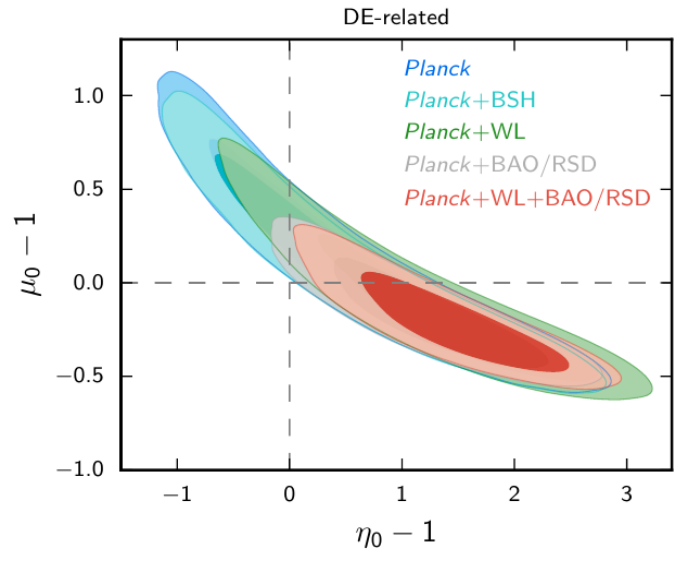
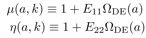
- Using Planck satellite data in 2015 and 2018, constraints were obtained on these two functions \(\mu\) and \(\eta\).
- Late-time parametrization: dependent on Dark Energy fraction
Planck 2015 results XIV, arXiv:1502.01590
Planck 2018 results VI, arXiv:1807.06209
Casas et al (2017), arXiv:1703.01271
Forecasts for Stage-IV surveys in:
Santiago Casas, 17.01.23
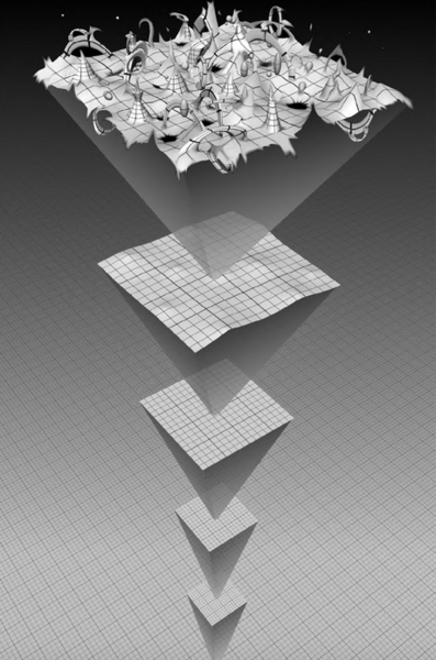
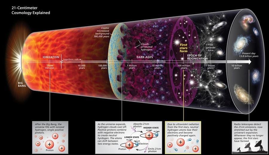
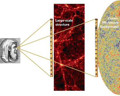
The Evolution of the Universe and the Dark Ages
Santiago Casas, 17.01.23
Complementarity of probes

21cm Intensity Mapping
Image credit: Sunayana Bhargava
Santiago Casas, 17.01.23
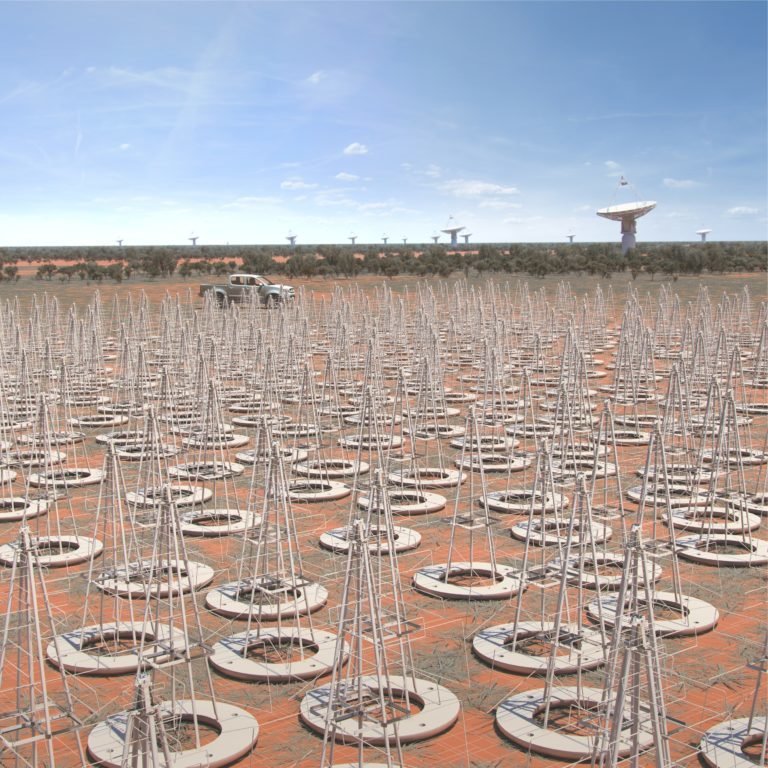
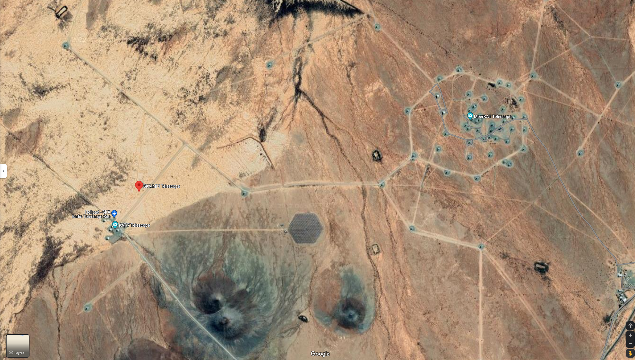
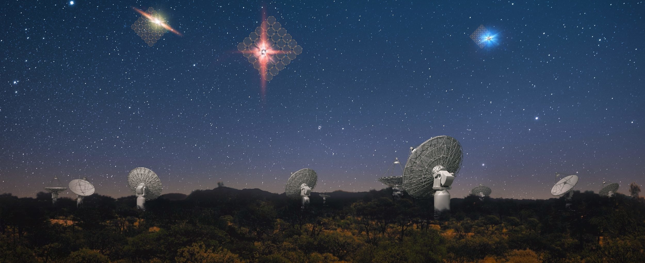
The Square Kilometer Array Obs. (SKAO)
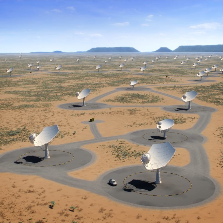
- SKA Phase 1: SKA1-Low and SKA1-Mid
- SKA1-Low: 130,000 dipole antennas, 65km max. baseline (Australia)
- SKA1-Mid: ~200 dishes of ~15m diameter, max. baseline 150km (South Africa)
- Precursors: ASKAP, MEERKAT, HERA...
Santiago Casas, 17.01.23
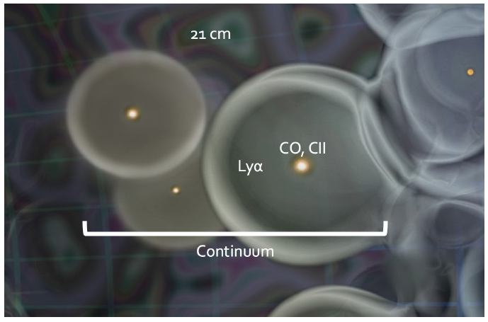
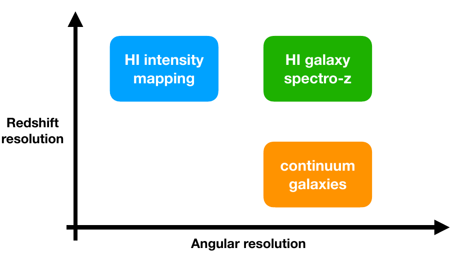
SKAO Probes
Image credit: Isabella Carucci
-
Continuum emission: Allows detection of position and shapes of galaxies.
-
Line emission of neutral Hydrogen (HI, 21cm):
-
Using redshifted HI line -> spectroscopic galaxy survey
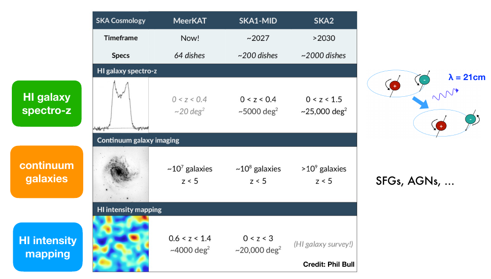
2. Intensity Mapping: Large scale correlations in HI brightness temperature -> very good redshift resolution,
good probe of structures

Santiago Casas, 17.01.23
SKAO Probes
Image credit: Isabella Carucci
-
Continuum emission: Allows detection of position and shapes of galaxies.
-
Line emission of neutral Hydrogen (HI, 21cm):
-
Using redshifted HI line -> spectroscopic galaxy survey
2. Intensity Mapping: Large scale correlations in HI brightness temperature -> very good redshift resolution,
good probe of structures
Santiago Casas, 17.01.23
SKAO GC Surveys
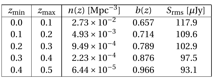
HI galaxies spectroscopic survey
- GCsp: HI galaxy spec. redshift survey: \(0.0 < z < 0.5\)
probes 3D matter power spectrum in Fourier space.
SKA1 Redbook 2018, arXiv:1811.02743
SKA1 Medium Deep Band 2: \(5000 \, \rm{deg}^2\)
Santiago Casas, 17.01.23
SKAO Angular Surveys
- GCsp: HI galaxy spec. redshift survey: \(0.0 < z < 0.5\)
probes 3D matter power spectrum in Fourier space -
GCco + WL + XCco (Continuum): \(0.0 < z < 3.0 \)
probes angular clustering of galaxies, Weak Lensing (Weyl potential) and galaxy-galaxy-lensing.
Angular number density:
\( n \approx 3.2 \rm{arcmin}^{-2}\)
SKA1 Redbook 2018, arXiv:1811.02743
Continuum galaxy survey
SKA1 Medium Deep Band 2: \(5000 \, \rm{deg}^2\)
Santiago Casas, 17.01.23
SKAO Angular Surveys
- GCsp: HI galaxy spec. redshift survey: \(0.0 < z < 0.5\)
probes 3D matter power spectrum in Fourier space - GCco + WL + XCco (Continuum): \(0.0 < z < 3.0 \)
probes angular clustering of galaxies, Weak Lensing (Weyl potential) and galaxy-galaxy-lensing.
Angular number density:
\( n \approx 3.2 \rm{arcmin}^{-2}\) - For comparison: Stage-IV:
\( n \approx 30 \rm{arcmin}^{-2}\)
*kindly provided by Stefano Camera
Continuum galaxy survey
SKA1 Medium Deep Band 2: \(5000 \, \rm{deg}^2\)
Santiago Casas, 17.01.23
Galaxy Clustering Recipe

BAO
Clustering
RSD
Spec-z
Euclid Collaboration, IST:Forecasts, arXiv: 1910.09273
Santiago Casas, 17.01.23
3x2pt recipe

Euclid preparation: VII. Forecast validation for Euclid cosmological probes. arXiv:1910.09273
Directly constrains MG function \(\Sigma\) through Weyl potential
Santiago Casas, 17.01.23
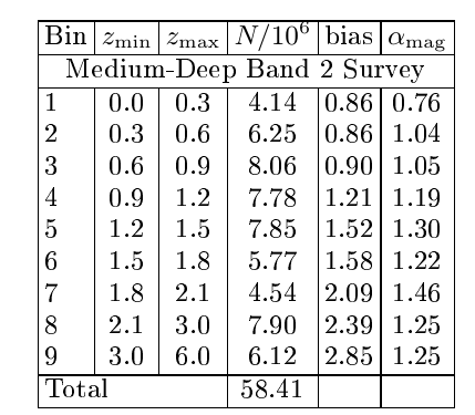
SKAO IM Surveys
- IM: Intensity mapping survey
\(0.4 < z < 2.5\) - Very good redshift resolution: \(\Delta z \approx \mathcal{O}(10^{-3}) \)
- We use: 11 redshift bins
-
Single dish mode:
\(N_d = 197\)
\(t_{obs} = 10000 \, \rm{hr} \)
We limit to the scales
\(0.001 < k < 0.25 \, [h/\rm{Mpc}] \)
SKA1 Medium Deep Band 1: \(20000 \,\rm{deg}^2\)
Santiago Casas, 17.01.23
Intensity Mapping
- IM probes the underlying matter power spectrum.
- Density bias given by the HI mass contained in dark matter halos.
- 21cm brightness temperature depends on cosmological background & the energy fraction of neutral Hydrogen in the Universe \(\Omega_{HI}\).
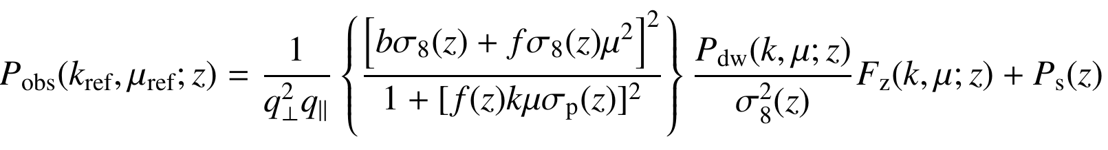
- \(P_{\delta\delta,zs}(z,k) \) is the redshift space matter power spectrum
\(P^{\rm IM}(z,k) = \bar{T}_{IM}(z)^2 \rm{AP}(z) K_{\rm rsd}^2(z, \mu; b_{\rm HI}) \)
\(FoG(z,k,\mu_\theta) \\ \times P_{\delta\delta,dw}(z,k) \)
\(\Omega_{HI} = 4(1+z)^{0.6} \times 10^{-4} \)
\( \bar{T}_{\mathrm{IM}}(z)= 189h \frac{(1+z)^2 H_0}{H(z)}\Omega_{HI}(z) \,\,{\rm mK} \)
Jolicoeur et al (2020) arXiv:2009.06197
Carucci et al (2020) arXiv:2006.05996
\( K_{\rm rsd}(z, \mu; b_{\rm HI}) = [b_{\rm HI}(z)^2+f(z)\mu^2] \)
\( b_{\rm HI}(z) = 0.3(1+z) + 0.6 \)
Santiago Casas, 17.01.23
Intensity Mapping x GCsp
- Cross correlation combines one term of brightness T with one K term for each "redshift sample".
- Same underlying matter power spectrum for both probes.
- A combined z-error (damping along the line of sight), where "sp" dominates, since the IM resolution is 1-2 orders of magnitude better.
\( b_{\rm g}(z) = \) fit to simulations for given galaxy sample
Jolicoeur et al (2020) arXiv:2009.06197
Wolz et al (2021) arXiv:2102.04946
\(\sigma_i(z) = \frac{c}{H(z)}(1+z) \delta_z\)
\(P^{{\rm IM} \times \rm{g}}(z,k) = \bar{T}_{\rm IM}(z) {\rm AP} (z) r_{\rm IM,opt} K_{\rm rsd}(z, \mu; b_{\rm HI}) \)
\( \times K_{\rm rsd}(z, \mu; b_{\rm g}) FoG(z,k,\mu_\theta) P_{\delta\delta,dw}(z,k) \)
\( \times \exp[-\frac{1}{2} k^2 \mu^2 (\sigma_{\rm IM}(z)^2+\sigma_{\rm sp}(z)^2)] \)
Santiago Casas, 17.01.23
Intensity Mapping
- \(P_{gg}\) underlying galaxy power spectrum.
- \(P_{IM}/T_{b}^2\): IM power spectrum.
- \(P_{IM,g}/T_{b}^2\) cross-spectrum.
- Angle-dependent beam effect is in the signal*, damps accross the l.o.s.
- Along the l.o.s. damping due to FoG, but higher amplitude due to Kaiser.
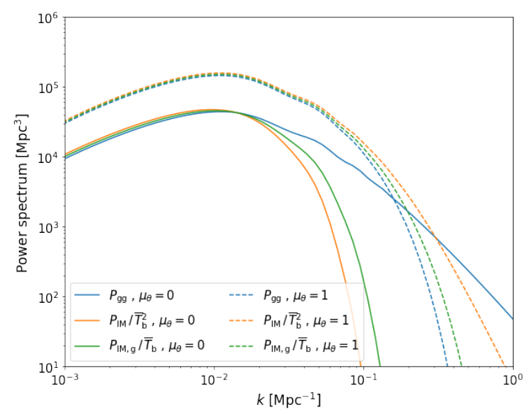
* Beam term in appendix
Santiago Casas, 17.01.23
Stage-IV surveys
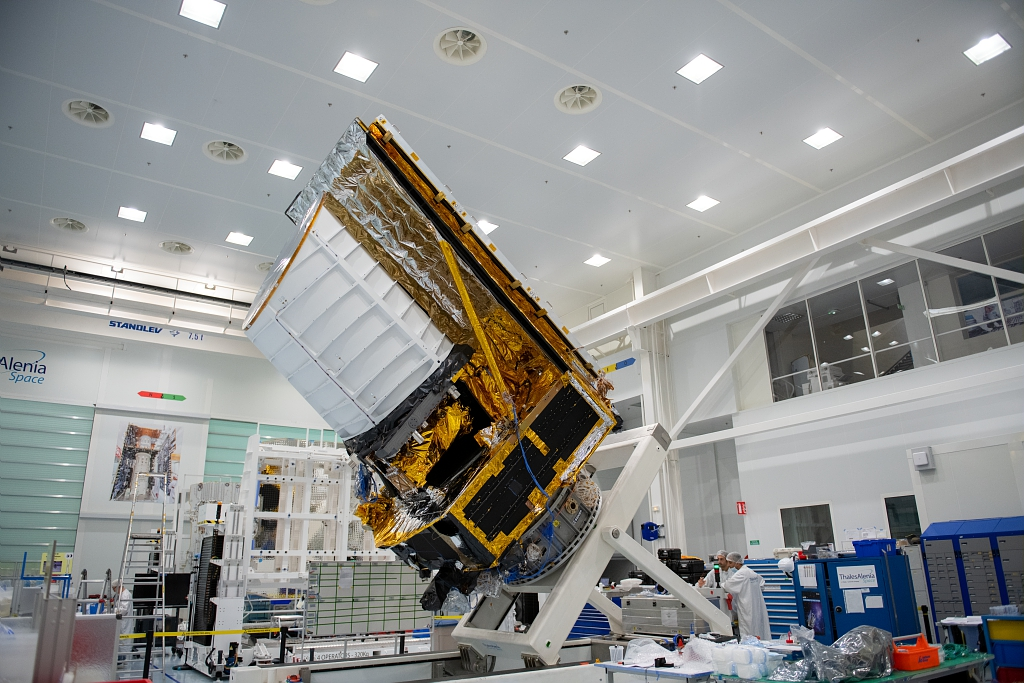
Euclid space satellite, now waiting in Cannes
Santiago Casas, 17.01.23
DESI telescope
- 14 000 square degrees in the sky
- 30 million accurate galaxy spectra
- Redshifts: 0 < z < 2
- Quasars up to z~3.5
- 5 years of observation

Specialized in Galaxy Clustering
Santiago Casas, 17.01.23
Vera Rubin Observatory
- Located in Chile, 8.4m telescope
- 20 billion galaxies
- Redshifts: 0 < z ~< 3
- 18,000 square degrees
- 11 years of observation
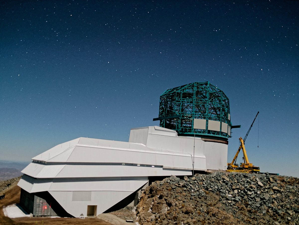
Specialized in Photometric Angular Probes: Lensing and Clustering
Santiago Casas, 17.01.23
Galaxy Clustering - IM Synergies

- GCsp-IM Cross-correlation in overlapping bins
- Addition in disjoint bins
- No GCsp-GCsp cross-correlation
Santiago Casas, 17.01.23
Fisher Matrix forecasts
Given a likelihood function L, representing the probability of the data d, given the model parameters \( \Theta\) , the Fisher matrix is defined as the Hessian of the L:
Assuming that L is a multivariate Gaussian distribution with a covariance matrix C independent of \(\Theta\) :
The explicit form of F, depends on the given observational probe and the physical model assumption, for example for GCsp:
Santiago Casas, 17.01.23
Fisher Matrix forecasts
What do we expect from the forecasts before doing them, just by looking at the formulas and the specs?
- SKAO (Phase1) has more independent probes but less statistical power (n(z) and area) -> less constraining power than Stage-IV
- WL and 3x2pt better at constraining \(\Sigma\)
- GCsp and IM better at constraining \(\mu\)
- GCsp x IM cross-corr. improves constraints on parameters?
Let's see the results !
Santiago Casas, 17.01.23
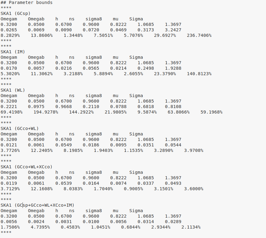
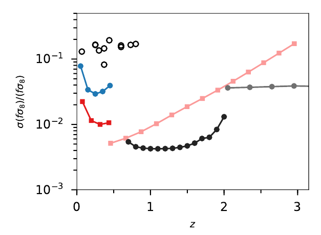
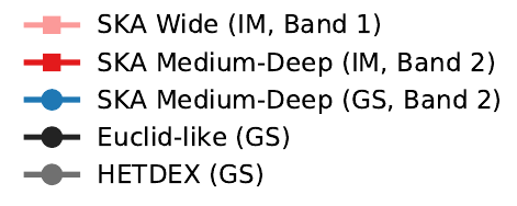
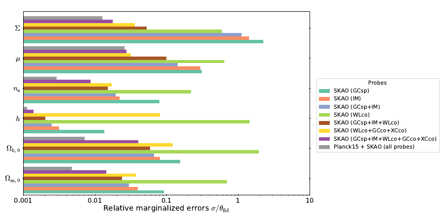
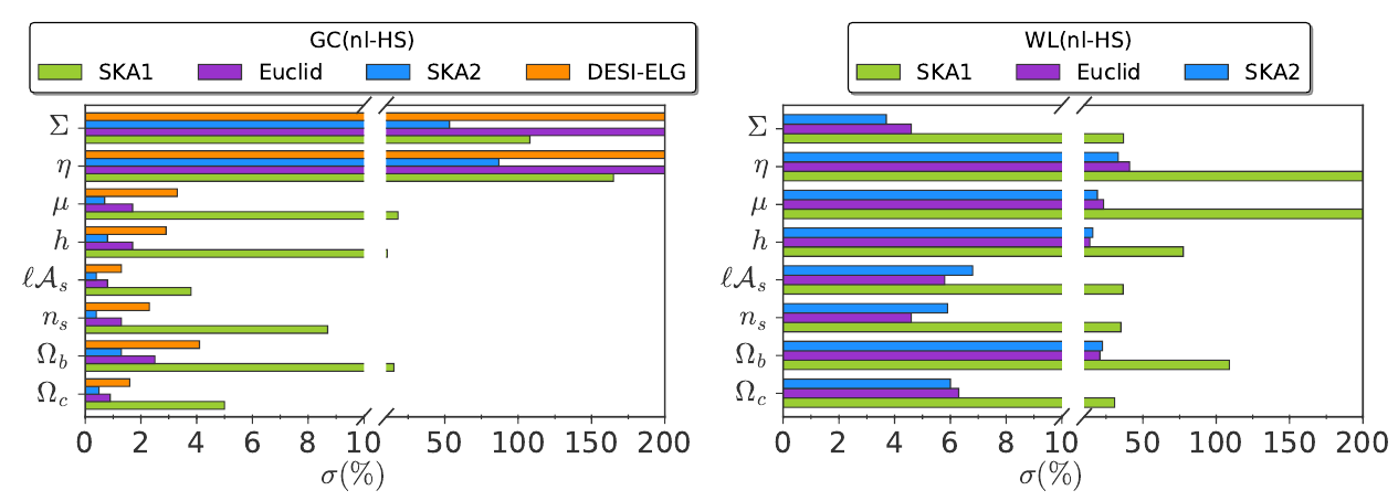
SKAO Results
- GC-IM probes measure \(\mu\) at small \(z\), where \(\mu\) becomes important.
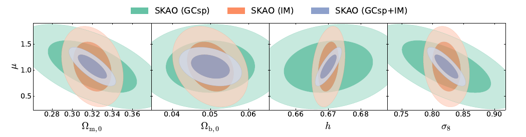
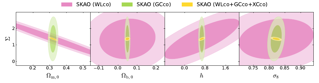
- Continuum probes measure better \(\Sigma\) ; Weyl potential is important.
Santiago Casas, 17.01.23
SKAO Results
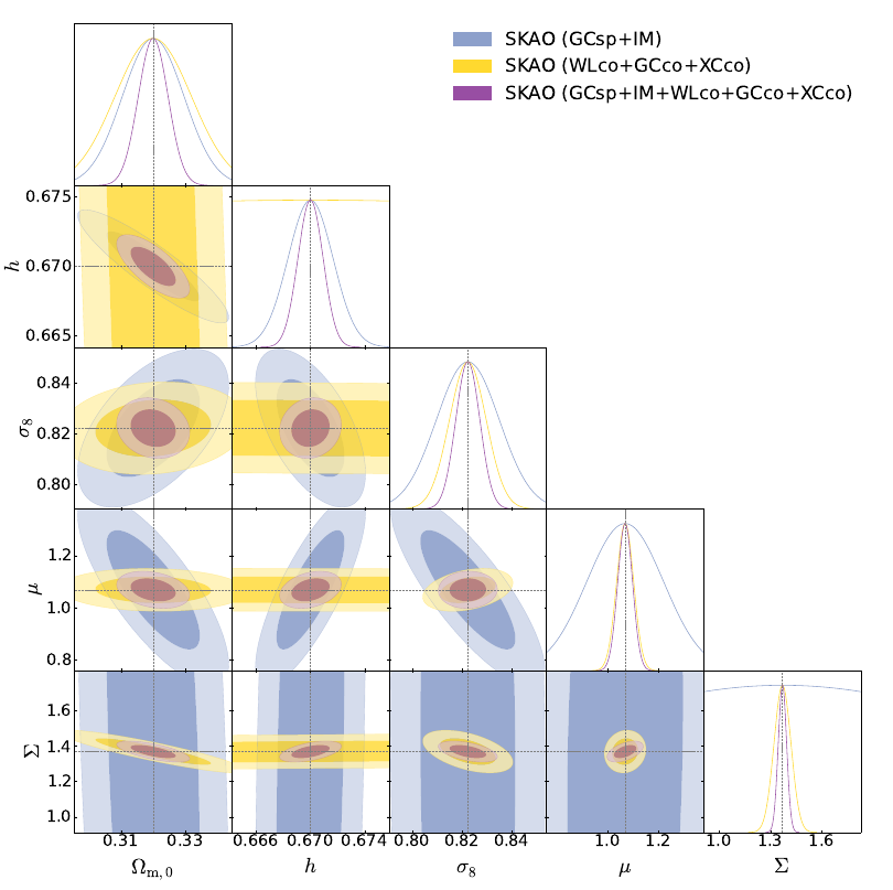
-
Blue: Combined GCsp+IM (3D)
- Yellow: Combined continuum probes (2D: angular)
- Purple: Combination of 3D and angular probes
- Constraints on \(\mu\) are good in angular, due to the XC contribution from GCco clustering.
Santiago Casas, 17.01.23
SKAO Results
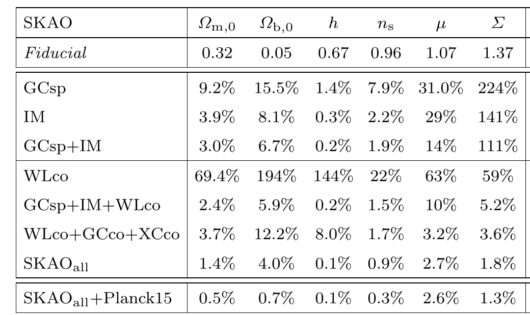
- Combining all SKAO probes (optimistic), 2-3% errors on \(\mu\) and \(\Sigma\).
- Minor improvement from Planck, mainly through ISW and CMB lensing.
Santiago Casas, 17.01.23
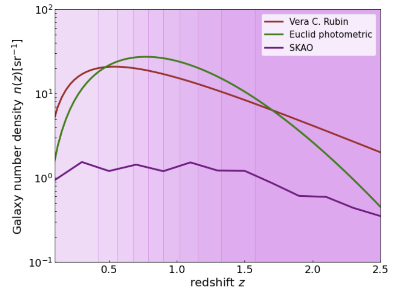
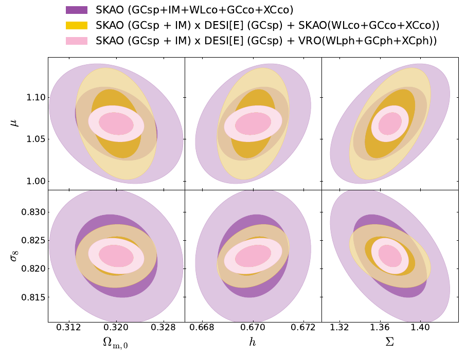
SKAO x DESI cross-correlation

- GCxIM probes do not improve constraints on MG parameters,
but improvement on \(h\) and \(\sigma_8\)
DESI_E : high-z Emission Line Galaxies
DESI_B: low-z Bright Galaxy Sample
SKAO GCsp: low-z HI Galaxies
Santiago Casas, 17.01.23
SKAO x DESI cross-correlation
- However, when combined with angular probes, there is a larger gain.
Santiago Casas, 17.01.23
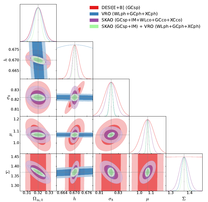
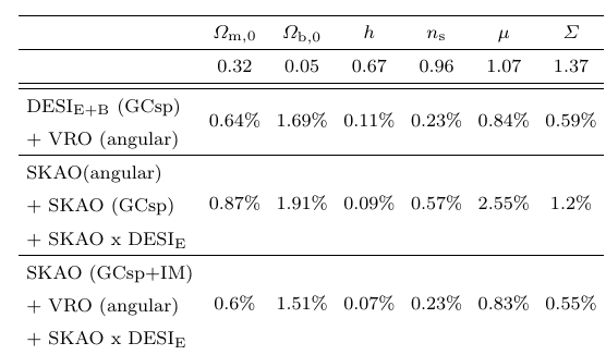
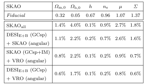
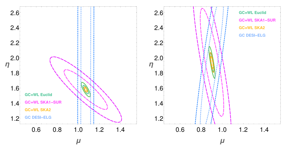
SKAO + optical
- SKAO + one Stage-IV survey is as competitive as two Stage-IV surveys together
- SKAO(all) better than DESI at constraining \(\mu\) and especially \(\Sigma\)
- SKAO(all) better than VRO at constraining \( h \)
- SKAO(spectro) + VRO, as good as DESI+VRO
- SKAO(spectro) x DESI + VRO has the maximum constraining power
Santiago Casas, 17.01.23
SKAO + optical
- SKAO + one Stage-IV survey is as competitive as two Stage-IV surveys
Santiago Casas, 17.01.23
Text
Conclusions
- \(\Lambda\)CDM is still the best fit to observations, however certain theoretical uncertainties and tensions in data are still of concern.
- Constraining modifications of gravity at the level of perturbations -> hints for alternative models.
- SKAO will be able to probe weak lensing and matter density perturbations in novel and independent ways compared to optical surveys.
- This will place constraints on deviations of standard gravity at yet unexplored redshifts.
- Synergies with optical surveys, like Euclid, DESI and Rubin, including cross-correlations are promising to remove systematics and break degeneracies.
- Using the good z-resolution of SKAO HI IM could place tight constraints on redshift-binned parametrizations.
Backup slide
Santiago Casas
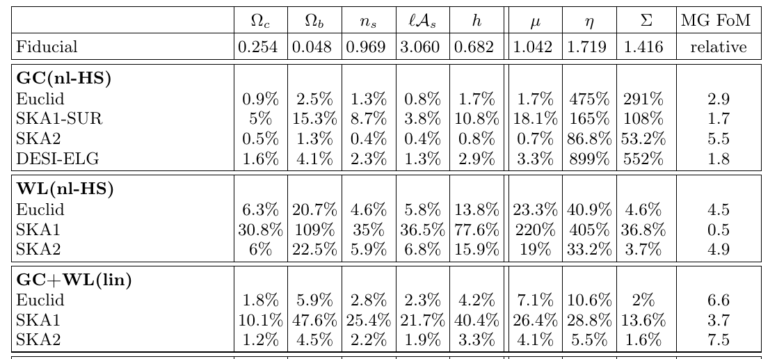
SKA1 vs Euclid
SKA1:
GC+WL+XC (Continuum) +
IM (HI 21cm) + GCsp(HI)
vs
Euclid
(Gcsp+GCph+WL+XCph)
vs
Euclid
(Gcsp+GCph+WL+XCph)+SKA1 Pk-probes.
Unfortunately, the \(\mu\) constraints from Euclid alone dominate over the improvement that SKA1 "Pk-probes" add
PRELIMINARY

Backup slide
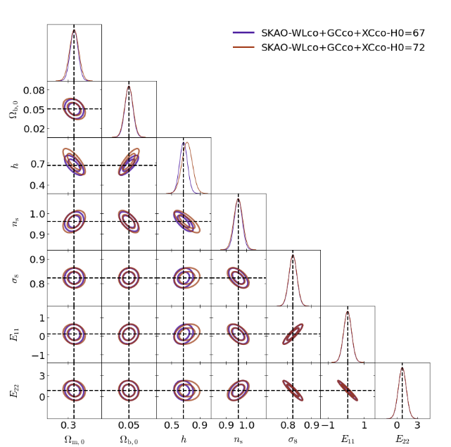
Testing at higher H0 value
Santiago Casas, 06.12.22
Late-time: Old SKA1, Euclid forecasts
Casas et al (2017), arXiv:1703.01271
- Old SKA1 forecasts contain only WL continuum and GCsp from HI galaxies
- Linear GCsp formalism and no IA params in WL
Santiago Casas, 06.12.22
Late-time: Old SKA1, Euclid forecasts
Casas et al (2017), arXiv:1703.01271
- However, we do roughly recover the same contour orientations and constraints with the new WL SKA1 forecasts.
- Deeply non-linear Pk recipe is the same, using an interpolation to recover GR at small scales.

Santiago Casas, 02.11.21
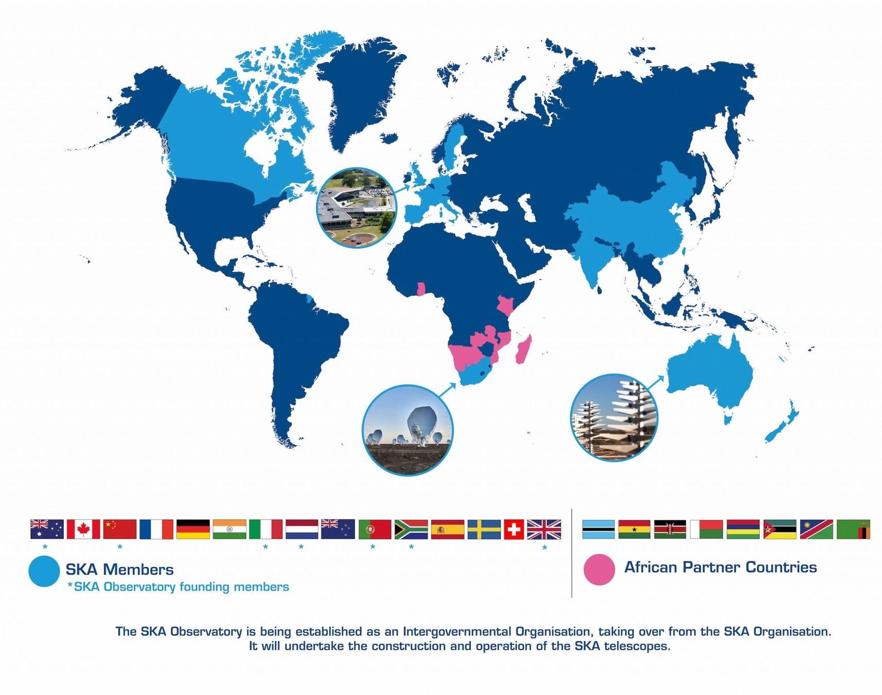
The Square Kilometer Array Obs. (SKAO)
- Next-generation Radioastronomy observatory
- Largest radiotelescope in the world: eventually 1km^2 area.
- 15 countries + partners
- Australia + South Africa installations
- ~2 billion Euros up to 2030.
- 5Tbps data rate and 250 Pflops needed for computation
Santiago Casas, 06.12.22
The Square Kilometer Array Obs. (SKAO)
- 15,000-20,000 square degrees in the sky
- Precursors: 10^7, SKA-phase1: 10^8, SKA-phase2: 10^9 galaxies
- SKA1-MID: 0 < z < 3
- SKA1-Low: 3 < z < ~ 20
- Cosmology is just one small area, Exoplanets, Craddle of Life, Reionization, Cosmic Magnetism....
Santiago Casas, 06.12.22
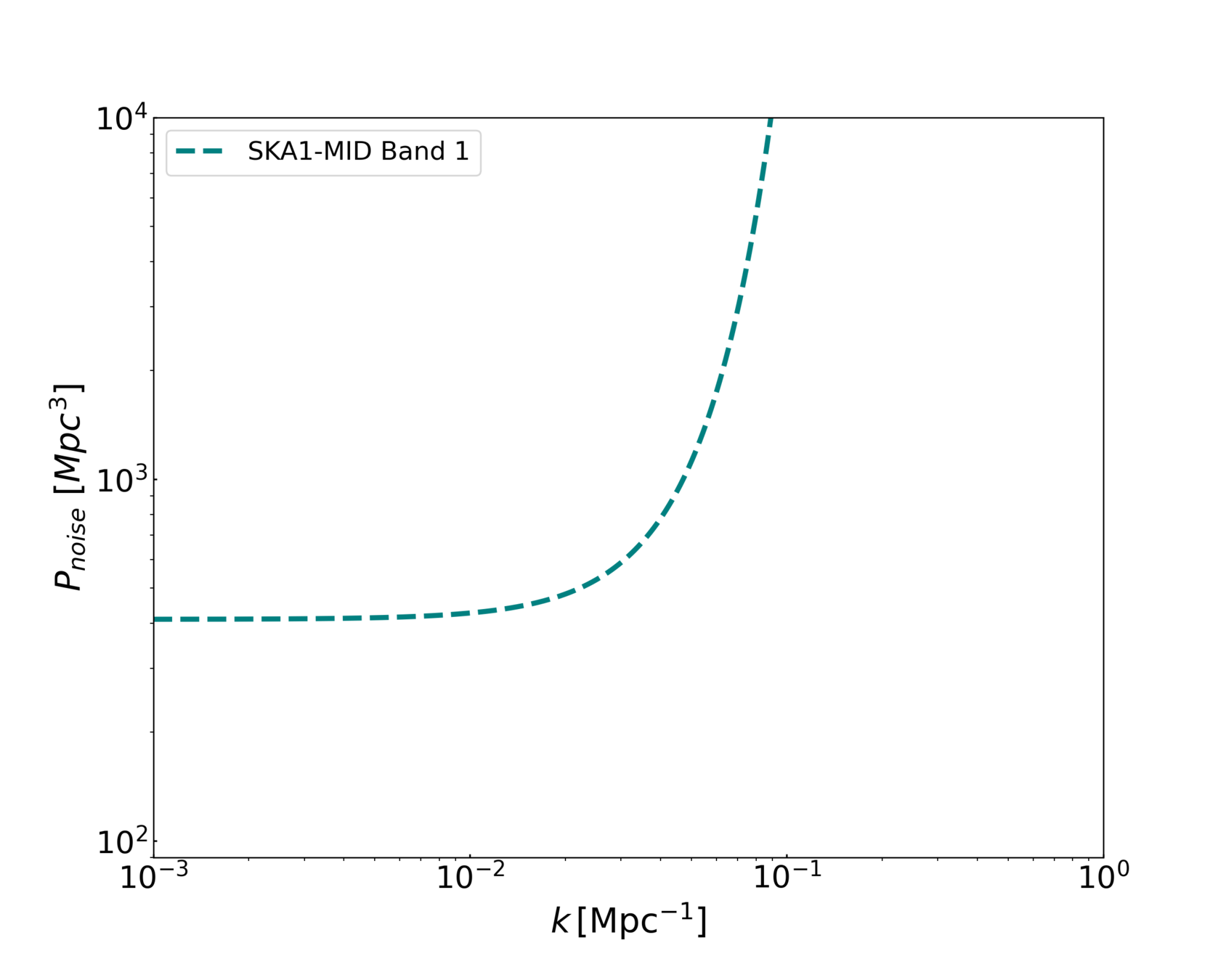
Intensity Mapping Noise Terms
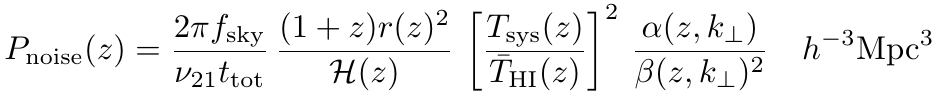
Number of dishes
Effective beam
\(\beta_{SD} = \exp[-\frac{k_\perp r(z)^2 \theta_b (z)^2}{8 \ln 2}] \)
\( \alpha_{SD} = \frac{1}{N_d} \)
Jolicoeur et al (2020) arXiv:2009.06197
Backup slide
Backup slide
Backup slide
Backup slide