Lesson 8:
Gaussian Mixture Model
Contents
- Introduction
- Properties of Gaussian Distribution
- Gaussian Mixture Model
- Properties of The Gaussian Mixture Model
- Training The Gaussian Mixture Model
Last Lecture: Gaussian Model
Assumes that the PDF of random variables have normal (Gaussian) distribution
$$\mathcal{N}(\vec{y};~\vec{\mu}, \Sigma)$$
- Models the conditional dependencies of all features \(f_i(y)\) via covariance matrix \(\Sigma\)
- Can't model complex non-Gaussian distributions
Introduction
Introduction
Today: Gaussian Mixture Model
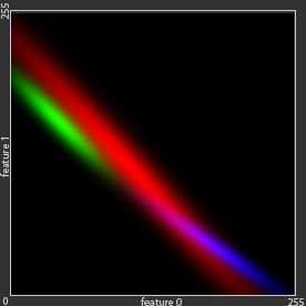
Assumes that the PDF of random variables can be modeled by a linear combination of multiple Gaussians $$\sum_i\mathcal{N}_i(\vec{y};~\vec{\mu}_i, \Sigma_i)$$
- Can model complex non-Gaussian distributions
- One of the most accurate methods among generative approaches
Expected Value
The average value of a random function \(f(x)\) under a probability distribution \(p(x)\) is called the expectation of \(f(x)\) and denoted through \(E[f(x)]\):
- Discrete case
$$E[f(x)]=\sum p(x)f(x)$$
- Continuous case
$$E[f(x)]=\int\limits^{\infty}_{-\infty}p(x)f(x)dx$$
Variance
The variance of a random function \(f(x)\) is the expected value of the squared deviation from the mean of \(f(x)\),
here mean \(\mu=E[f(x)]\)
$$Var[f(x)]=E[(f(x)-E[f(x)])^2]$$
- The expression for the variance can be expanded as follows
$$E[(f(x)-E[f(x)])^2]=E[f(x)^2]-E[f(x)]^2$$
Properties of
The Gaussian
Distribution
1. Expected Value
If a random variable \(y\) has normal distribution:
- \(p(y)=\mathcal{N}(y;~\mu, \sigma)\)
- \(f(y)=y\)
2. Variance
Gaussian Mixture Model
Mixture of Gaussians
- The Gaussian distribution is the most commonly found in nature, it suffers from the lack of generality
- It has obvious limitations when it comes to approximating complex distributions. Whereas a linear
superposition of number of Gaussians is free from these limitations and in most cases can give us a
better characterisation of a data set
- Such superpositions, formed by taking linear combinations of more basic distributions such as
Gaussians, can be formulated as probabilistic models known as mixture distributions
- By using a sufficient number of Gaussians, and by adjusting their means and covariances as well as the
coefficients in the linear combination, almost any continuous density can be approximated to arbitrary
accuracy
We therefore consider a superposition of \(G\) Gaussian densities of the form:
$$\mathcal{P}(\vec{y}) = \sum^{G}_{k=1}\omega_k\mathcal{N}_k(\vec{y};~\vec{\mu}_k,\Sigma_k)$$
which is called a mixture of Gaussians.
Each Gaussian density \(\mathcal{N}_k(\vec{y};~\vec{\mu}_k,\Sigma_k)\) is called a mixture component of the mixture and has its own mean \(\vec{\mu}_k\) and covariance \(\Sigma_k\)
The weights \(\omega_k\) are called mixture coefficients
Examples
The Gaussian mixture distribution in 1D formed by 3 Gaussians
$$\mathcal{P}(y)=\omega_1\mathcal{N}_1+\omega_2\mathcal{N}_2 + \omega_3\mathcal{N}_3$$
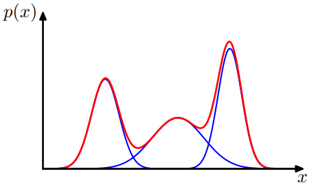
Source: Christopher M. Bishop's textbook “Pattern Recognition & Machine Learning”
Examples
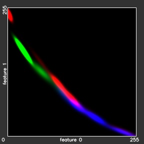
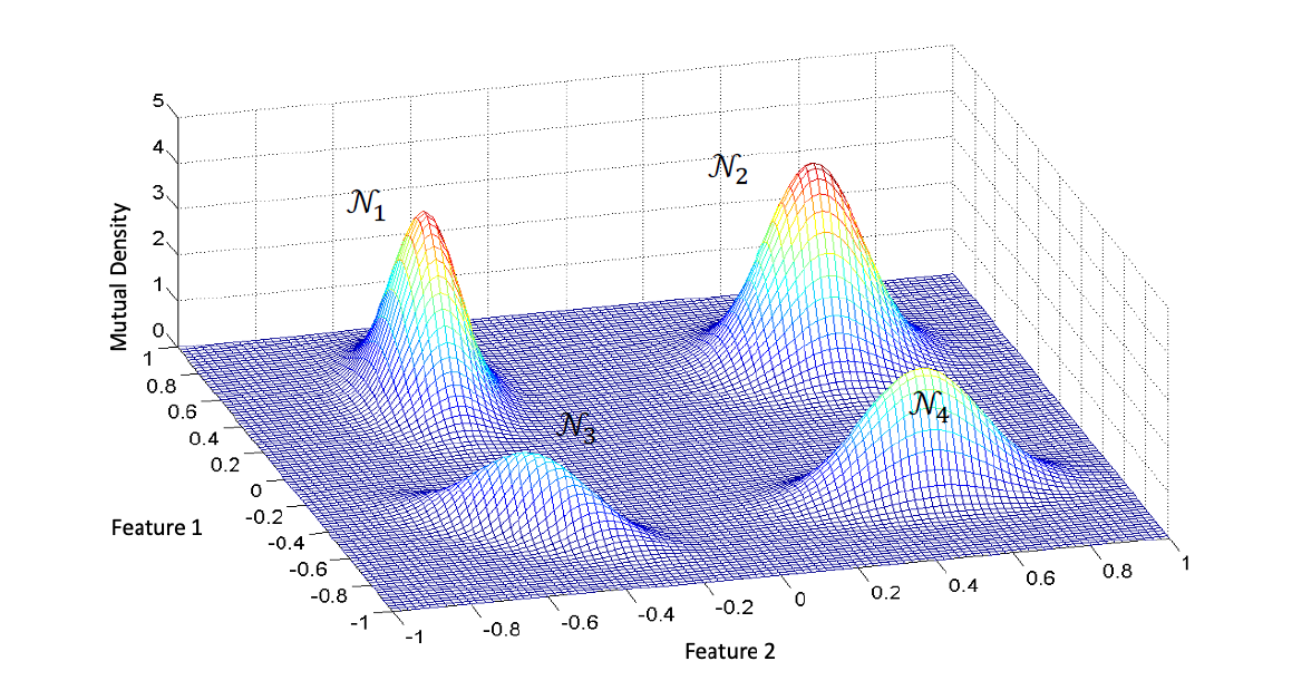
The Gaussian mixture distribution in 2D formed by 4 Gaussians
$$\mathcal{P}(\vec{y})=\omega_1\mathcal{N}_1+\omega_2\mathcal{N}_2 + \omega_3\mathcal{N}_3+\omega_4\mathcal{N}_4$$
Complexity
- All samples with correlation (real world):
$$256^{nFeatures}\cdot nStates = 256^2\cdot3$$
- Bayes model - no correlation:
$$256\cdot nFeatures\cdot nStates = 256\cdot 2 \cdot 3$$
- Gaussian model with correlation:
$$(nFeatures^2 + nFeatures)\cdot nStates = (4 + 2)\cdot 3$$
- Gaussian mixture model with correlation:
$$nGaussians\cdot(nFeatures^2 + nFeatures + 1)\cdot nStates = nGaussians\cdot(4 + 2 + 1)\cdot 3$$
Properties of
The Gaussian Mixture Model
Mixture Coefficients
If we integrate both sides of equation
\(\mathcal{P}(\vec{y}) = \sum^{G}_{k=1}\omega_k\mathcal{N}_k(\vec{y};~\vec{\mu}_k,\Sigma_k)\) with respect to \(\vec{y}\), and note that both \(\mathcal{P}(\vec{y})\) and the individual Gaussian components are normalised, we obtain \(\sum^{G}_{k=1}\omega_k=1\).
Also, given that \(\mathcal{N}_k(\vec{y};~\vec{\mu}_k, \Sigma_k)\ge0\), a sufficient condition for the requirement \(\mathcal{P}(\vec{y})\ge0\) is that \(\omega_k\ge0, \forall k \in [1; G]\). Combining this with the condition above we obtain \(0\le\omega_k\le1\).
Mixture Coefficients
We therefore see that the mixture coefficients satisfy the requirements to be probabilities, and so, could be considered as as the prior probabilities of picking the k-th component.
The densities \(\mathcal{N}_k(\vec{y};~\vec{\mu}_k, \Sigma_k)\), in its turn, could be considered as the probabilities of \(\vec{y}\) conditioned on \(k\): \(p(\vec{y}~|~k)\).
From Bayes' theorem we can write:
$$p(\vec{y}~|~k)\propto p(\vec{y})\cdot p(\vec{y}~|~k) = \omega_k\mathcal{N}_k(\vec{y};~\vec{\mu}_k,\Sigma_k)$$
Training
The Gaussian Mixture Model
Training The Mixture Model
(a non-trivial task)
is the estimation of mixture coefficients \(\omega_k\) and parameters of the mixture components \(\vec{\mu}_k\), \(\Sigma_k\) from training dataset
- In some extent, this problem could be simplified to a problem of finding clusters in a set of training data points, which could be solved, for example, by using a non-probabilistic technique called the K-means algorithm.
- The goal of this algorithm is to partition the training data set into some number \(K\) of clusters. Intuitively, we might think of a cluster as a comprising a group of data points whose inter-point distances are small compared with the distances to points outside of the cluster.
- But a more general probabilistic technique for finding maximum likelihood estimators is the expectation maximization algorithm.
Training The Mixture Model
(a non-trivial task)
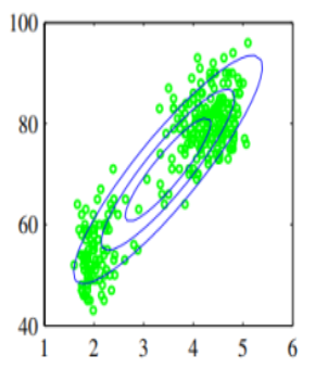
The green dot are an example of given data that cannot be modelled using single Gaussian distribution, because it has two clusters or summits.
To model green dots distributions, we can use linear combination of Gaussian distributions , which is much better than single Gaussian distribution.
