Lesson 1:
Introduction to Probability Theory
Contents
- Introduction to Probability Theory
- Two fundamental rules of Probability Theory
- Main properties of probabilities
- Bayes Law
Probability Theory
is the branch of mathematics concerned with analysis of random phenomena
- The study of probability helps us figure out the likelihood of something happening
- In mathematics we call this "something happening" or an "event"
Introduction
Probability
is a way of expressing what the chances are that an event will occur
- Numerically probability \(p\) is expressed with a real-valued number between 0 and 1: $$p\in[0;1]$$
- Such number represents the chance from 0% to 100%
Random Variable
is a variable \(v\) whose values depend on
outcomes of a random phenomenon
Discrete Random Variable
deal with events that occur in a countable sample space
- countable number of states (outcomes of the random event) $$v\in\{s_1, s_2,\dots,s_n\}$$
- usually has non-zero probability for each state \(s_i\)$$p(v=s_i)\geq0$$
- sum of the probabilities for all states is always 100% $$\displaystyle\sum_i{p(v=s_i)}=1$$
Continuous Random Variable
deal with events that occur in a continuous sample space
- infinite number of states $$v\in[a;d]$$
- probability for each concrete state \(c\) is infinitely small $$p(v=c)=0$$
- instead, the probabilities of \(v\) to be in some interval are evaluated $$p(b< v\leq c)\geq0,$$ $$p(a< v\leq d)=1$$
Discrete Random Variable
- countable number of states (outcomes of the random event) $$v\in\{s_1, s_2,\dots,s_n\}$$
- usually has non-zero probability for each state \(s_i\)$$p(v=s_i)\geq0$$
- sum of the probabilities for all states is always 100% $$\displaystyle\sum_i{p(v=s_i)}=1$$
Thus, the probability \(p\) of one discrete random variable (event) \(v\) which is defined for \(n\) states comprises \(n\) chances for every state $$p(v) \equiv \left\{p(v=s_1), p(v=s_2),\dots,p(v=s_n)\right\}$$
In the DGM library such probabilities are stored as vectors of floating-point numbers:
std::vector<float> probability;
Two Fundamental Rules of Probability Theory
1. Sum Rule
Here \(p(v_1,v_2)\) is a joint probability and is verbalised as
the probability of \(v_1\) and \(v_2\)
Joint Probability
In DGM library this is a two-dimensional matrix whose size is equal to the number of states of each of the random variables and the value of each element is equal to the probability of events \(v_1\) and \(v_2\) occurring simultaneously
cv::Mat probability(n, m, CV_32FC1);
Joint probability is commutative: $$p(v_1,v_2)=p(v_2,v_1)$$
2. Product Rule
Here the quantity \(p(v1~|~v_2)\) is a conditional probability and is verbalised as
the probability of \(v_1\) given \(v_2\)
Conditional Probability
In DGM library this is a two-dimensional matrix whose size is equal to the number of states of each of the random variables and the value of each element is equal to the probability of event \(v_1\) occurring, provided event \(v_2\) has occurred
cv::Mat probability(n, m, CV_32FC1);
Conditional probability is not commutative: $$p(v_1~|~v_2)\not=p(v_2~|~v_1)$$
Main Properties of Probabilities
Statistical Independence
Two random variables \(v_1\) and \(v_2\) are statistically independent (also unconditional independent) if and only if
$$p(v_1~|~v_2)=p(v_1)$$
As consequence we have:
Statistical Independence
Two random variables \(v_1\) and \(v_2\) are statistically independent (also unconditional independent) if and only if
$$p(v_1~|~v_2)=p(v_1)$$
As consequence we have:
Conditional Independence
Two random variables \(v_1\) and \(v_2\) are conditional independent given a third random variable \(v_3\) if and only if
$$p(v_1~|~v_2, v_3)=p(v_1~|~v_3)^1$$
As consequence we have:
\(^1\)This notation is equivalent to \(v_1\perp\!\!\!\perp v_2~|~v_3\)
Conditional Independence
Two random variables \(v_1\) and \(v_2\) are conditional independent given a third random variable \(v_3\) if and only if
$$p(v_1~|~v_2, v_3)=p(v_1~|~v_3)^1$$
As consequence we have:
\(^1\)This notation is equivalent to \(v_1\perp\!\!\!\perp v_2~|~v_3\)
which must be hold for every possible value of \(v_3\), and not just for some values
General Product Rule
By application of the product rule of probability
\(p(v_i,v_j)=p(v_i~|~v_j)\cdot p(v_j)\), we can write the joint distribution for an arbitrary number \(n\) of random variables \(\vec{v} = (v_1,\dots,v_n)^\top\)
Note, that this decomposition holds for any choice of the joint distribution
or

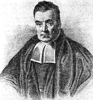
Thomas Bayes
c. 1701 - 7 April 1761
British mathematician and priest
Portrait purportedly of Bayes used in a 1936 book, but it is doubtful whether the portrait is actually of him. No earlier portrait or claimed portrait survives
Bayes Law
Bayes law may be derived directly from the product rule and the commutative property of joint probability:
$$p(v_1,v_2)=p(v_1~|~v_2)\cdot p(v_2)$$
$$p(v_2,v_1)=p(v_2~|~v_1)\cdot p(v_1)$$
$$p(v_1,v_2)=p(v_2,v_1)\Longrightarrow p(v_1~|~v_2)\cdotp(v_2) = p(v_2~|~v_1)\cdot p(v_1)$$

Thomas Bayes
c. 1701 - 7 April 1761
British mathematician and priest
Portrait purportedly of Bayes used in a 1936 book, but it is doubtful whether the portrait is actually of him. No earlier portrait or claimed portrait survives
Bayes Law
Bayes law may be derived directly from the product rule and the commutative property of joint probability:
Posterior probability
Likelyhood
Prior probability
"Bayes law for probability theory, the same as Pythagorean theorem for geometry"
-Harold Jeffreys, British mathematician
Total probability

Thomas Bayes
c. 1701 - 7 April 1761
British mathematician and priest
Portrait purportedly of Bayes used in a 1936 book, but it is doubtful whether the portrait is actually of him. No earlier portrait or claimed portrait survives
Bayes Law
Bayes law may be derived directly from the product rule and the commutative property of joint probability:
Posterior probability
Likelyhood
Prior probability
Total probability
Total probability: $$p(B)=\displaystyle\sum^{n}_{i=1}{p(B|A_i)\cdot p(A_i)}$$
Allows to calculate the probability of an event of interest through conditional probabilities of this event in respect to the probabilities of some sypothesises
Example
Bayes Law
Bayes law may be derived directly from the product rule and the commutative property of joint probability:
Posterior probability
Likelyhood
Prior probability
- A school has 60% boys and 40% girls;
- The girl students wear trousers or skirts in equal numbers; the boys all wear trousers;
- An observer sees a student in trousers;
- What is the probability that the student is a girl ?
Formulating the task:
- Let event \(A\) denotes a girl, \(\bar{A}\) - a boy
- Let event \(B\) denotes trousers, \(\bar{B}\) - skirts
- Find \(p(A~|~B)\)
Total probability: $$p(B)=\displaystyle\sum^{n}_{i=1}{p(B|A_i)\cdot p(A_i)}$$
Allows to calculate the probability of an event of interest through conditional probabilities of this event in respect to the probabilities of some sypothesises
Total probability
Example
Bayes Law
Bayes law may be derived directly from the product rule and the commutative property of joint probability:
- A school has 60% boys and 40% girls;
- The girl students wear trousers or skirts in equal numbers; the boys all wear trousers;
- An observer sees a student in trousers;
- What is the probability that the student is a girl ?
Formulating the task:
- Let event \(A\) denotes a girl, \(\bar{A}\) - a boy
- Let event \(B\) denotes trousers, \(\bar{B}\) - skirts
- Find \(p(A~|~B)\)
$$p(B)=\displaystyle\sum^{n}_{i=1}{p(B|A_i)\cdot p(A_i)}$$