Lesson 5:
Shading
Contents
- Introduction
- Radiometry
- Rendering Equation
- The BRDF!
- BRDF Approximations
- Light Sources
Introduction
What is Light?
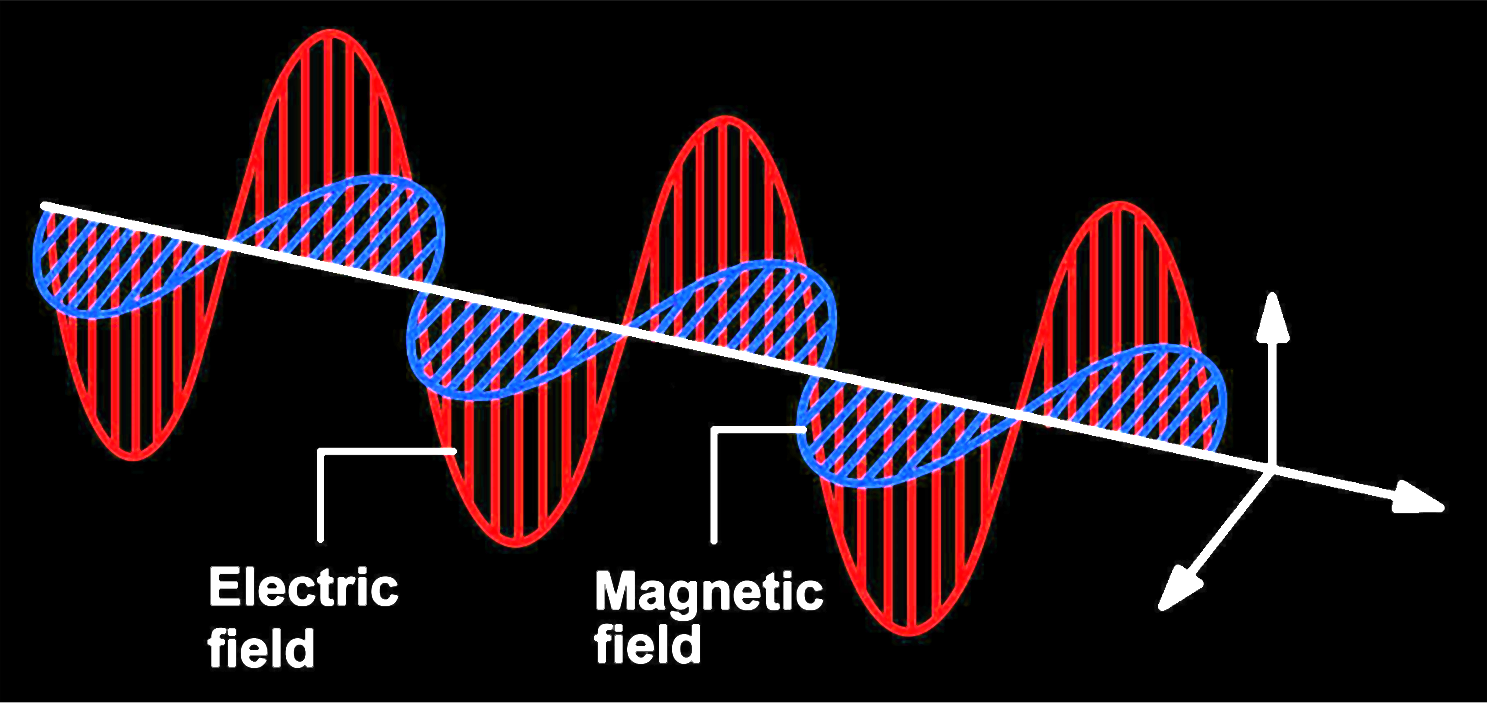
Electro-magnetic wave propagating at speed of light
Radiometry - the study of the propagation of electromagnetic radiation in an environment
Introduction
What is Light?
Introduction
What is Light?
Ray
- Linear propagation
- Geometric optics
Vector
- Polarisation
- Jones Calculus: matrix representation
Wave
- Diffraction, interference
- Maxwell equations: propagation of light
Particle
- Light comes in discrete energy quanta: photons
- Quantum theory: interaction of light with matter
Field
- Electromagnetic force: exchange of virtual photons
- Quantum Electrodynamics (QED): interaction between particles
Introduction
What is Light?
Light in Computer Graphics
- Linearity: The combined effect of two inputs to an optical system is always equal to the sum of the effects of each of the inputs individually
- Energy conservation: When light scatters from a surface or from participating media, the scattering events can never produce more energy than they started with
- No polarisation: We will ignore polarisation of the electromagnetic field; therefore, the only relevant property of light is its distribution by wavelength (or, equivalently, frequency)
- No fluorescence or phosphorescence: The behaviour of light at one wavelength is completely independent of light’s behaviour at other wavelengths or times
-
Steady state: Light in the environment is assumed to have reached equilibrium, so its distribution isn’t changing over time
(this happens nearly instantaneously with light in realistic scenes, so it is not a limitation in practice)
Ray
- Linear propagation
- Geometric optics
Radiometry
Basic Quantities
There are four radiometric quantities that are central to rendering
Flux
Irradiance
Intensity
Radiance
They can each be derived from energy by successively taking limits over time, area, and directions
Energy
Thus all of the radiometric quantities are in general wavelength dependent
Energy is measured in joules (\( J \)). Sources of illumination emit photons, each of which is at a particular wavelength and carries a particular amount of energy. All of the basic radiometric quantities are effectively different ways of measuring photons.
A photon at wavelength \( \lambda \) carries energy
$$ Q= \frac{hc}{\lambda},$$
where \( c \approx 3\times 10^8 m/s\) is the speed of light and \( h\approx 6,626\times 10^{-34} m^2kg/s \) is Planck's constant
Radiometry
Basic Quantities
There are four radiometric quantities that are central to rendering
Flux
Irradiance
Intensity
Radiance
Energy
$$ Q= \frac{hc}{\lambda},$$
Radiant power (Flux) is the total amount of energy passing through a surface or region of space per unit time. Radiant power can be found by taking the limit of differential energy per differential time:
$$ \Phi = \frac{dQ}{dt} $$
Its units are joules/second (\( J/s \)), or more commonly, watts (\( W \)). Total emission from light sources is generally described in terms of flux.
Note that the total amount of flux measured on either of the two spheres is the same - although less energy is passing through any local part of the large sphere than the small sphere, the greater area of the large sphere means that the total flux is the same.
Flux from a point light source measured by the total amount of energy passing through imaginary spheres around the light
Radiometry
Basic Quantities
There are four radiometric quantities that are central to rendering
Flux
$$ \Phi = \frac{dQ}{dt} $$
Irradiance
Intensity
Radiance
Energy
$$ Q= \frac{hc}{\lambda},$$
Irradiance (the area density of flux arriving at a surface), or radiant exitance (the area density of flux leaving a surface) is the average density of power over the area over which photons per time is being measured:
$$ E=\frac{\Phi}{A} $$
Its units are \( W/m^2 \).
Flux from a point light source measured by the total amount of energy passing through imaginary spheres around the light
More generally, we can define irradiance by taking the limit of differential power per differential area at a point \( p \):
$$ E(p) = \lim_{\Delta A \rightarrow 0} \frac{\Delta\Phi(p)}{\Delta A} = \frac{d\Phi(p)}{dA}$$
Radiometry
Basic Quantities
There are four radiometric quantities that are central to rendering
Flux
$$ \Phi = \frac{dQ}{dt} $$
Irradiance
Intensity
Radiance
Energy
$$ Q= \frac{hc}{\lambda},$$
Lambert’s Law: Irradiance arriving at a surface varies according to the cosine of the angle of incidence of illumination, since illumination is over a larger area at larger incident angles.
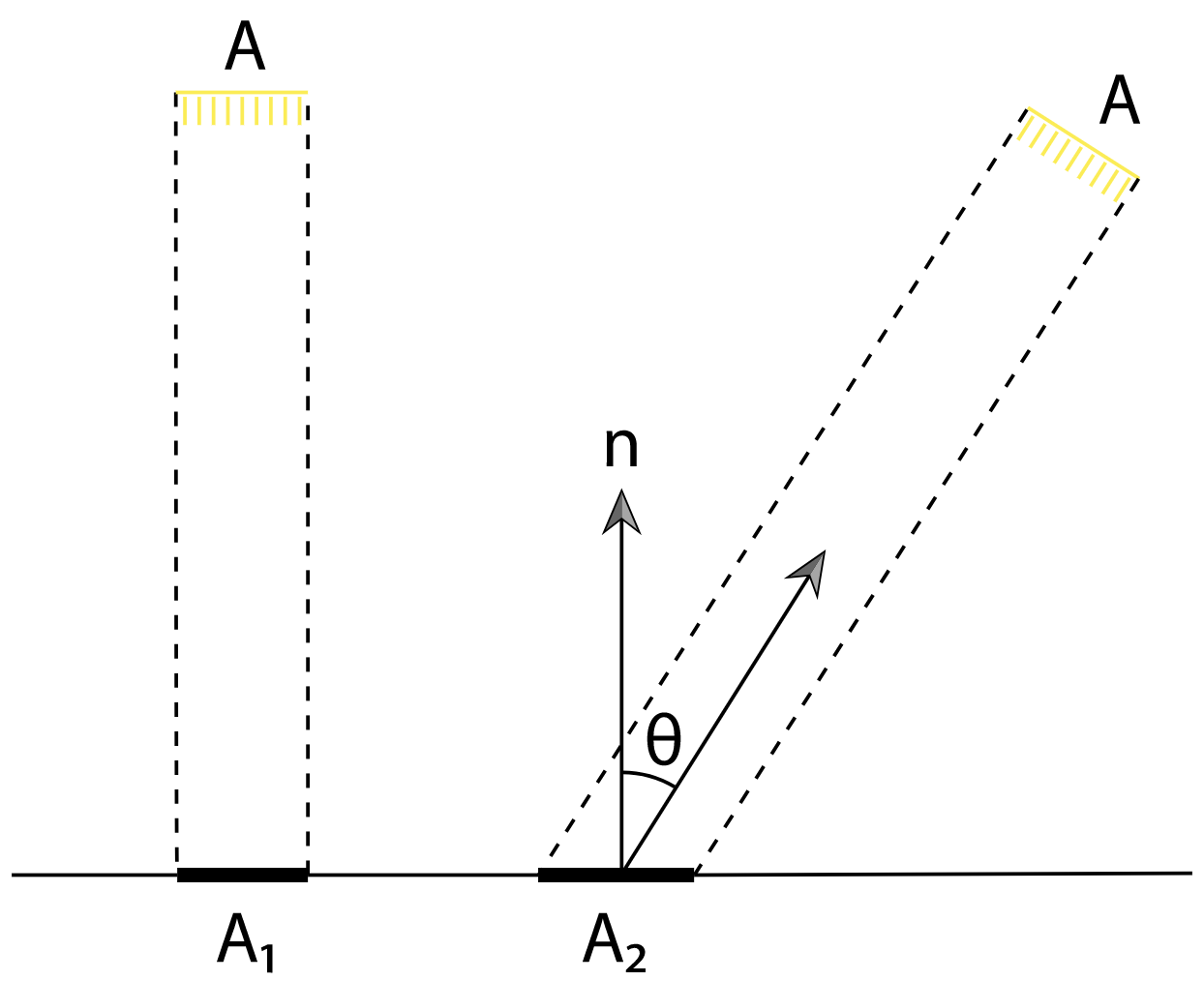
Consider a light source with area \(A\) and flux \(\Phi\) that is illuminating a surface. If the light is shining directly down on the surface, then the area on the surface receiving light \(A_1\) is equal to \(A\). Irradiance at any point inside \(A_1\) is then \(E_1=\frac{\Phi}{A}\)
However, if the light is at an angle to the surface, the area on the surface receiving light is larger. If \(A\) is small, then the area receiving flux, \(A_2\) , is roughly \(A/\cos\Theta\). For points inside \(A_2\), the irradiance is therefore \(E_2=\frac{\Phi\cos\Theta}{A}\)
Irradiance (the area density of flux arriving at a surface), or radiant exitance (the area density of flux leaving a surface) is the average density of power over the area over which photons per time is being measured:
$$ E=\frac{\Phi}{A} $$
Its units are \( W/m^2 \).
Radiometry
Basic Quantities
There are four radiometric quantities that are central to rendering
Flux
$$ \Phi = \frac{dQ}{dt} $$
Irradiance
$$ E=\frac{\Phi}{A} $$
Radiance
Energy
$$ Q= \frac{hc}{\lambda},$$
Intensity | Solid Angle
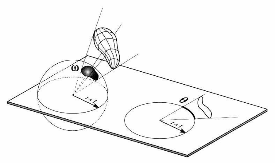
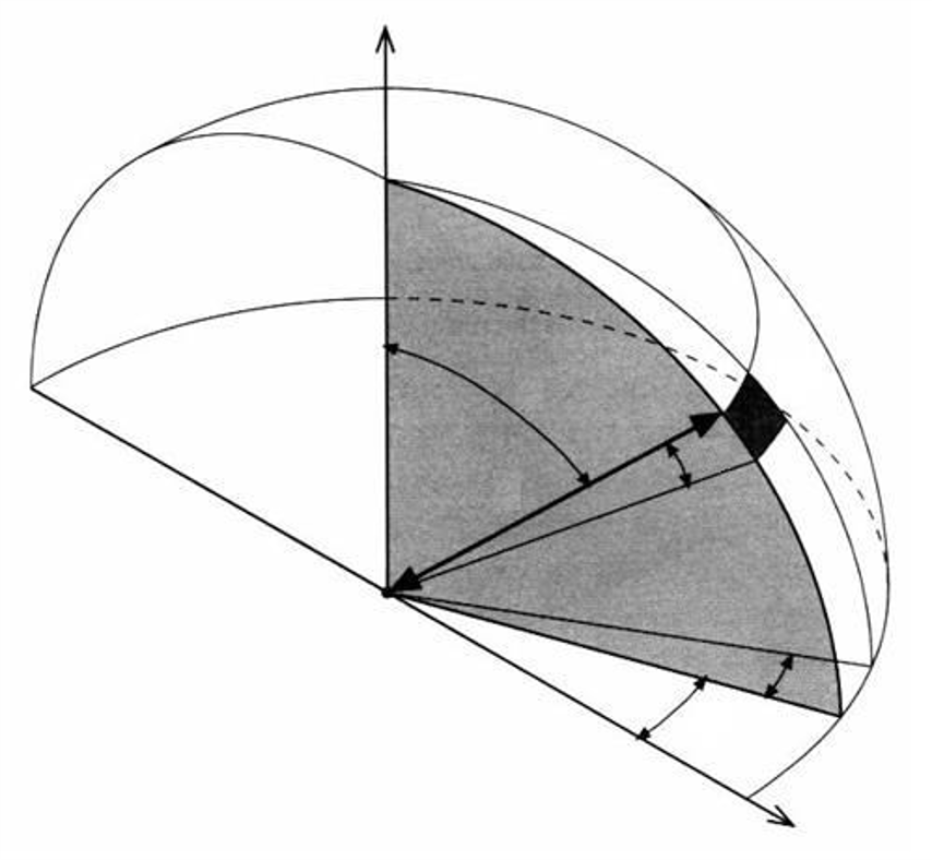
Planar angle
The planar angle \(\theta\) is the total angle subtended by some object with respect to some position.
If we project a shaded object onto a unit circle, some length of the circle \(l\) will be covered by its projection. The arc length (\(l=\theta\)) is the angle subtended by the object.
Planar angles are measured in radians.
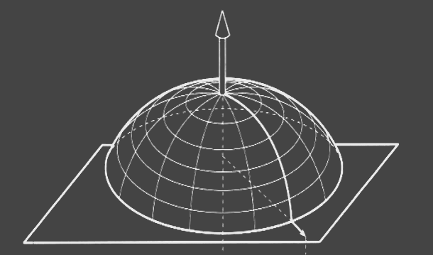
Solid angle
The solid angle \(\omega\) extends the 2D unit circle to a 3D unit sphere. The total area \(s\) is the solid angle subtended by the object.
Solid angles are measured in steradians [\(sr\)].
The entire sphere subtends a solid angle of \(4\pi sr\), and a hemisphere subtends \(2\pi sr\).
Radiometry
Basic Quantities
There are four radiometric quantities that are central to rendering
Flux
$$ \Phi = \frac{dQ}{dt} $$
Irradiance
$$ E=\frac{\Phi}{A} $$
Radiance
Energy
$$ Q= \frac{hc}{\lambda},$$
Intensity | Solid Angle
Intensity is the angular density of emitted power. For an infinitesimal light source surrounded with a unit sphere, we can compute the angular density of emitted power over the entire sphere of directions:
$$ I=\frac{\Phi}{4\pi} $$
Its units are \( W/sr \). But more generally we are interested in taking the limit of a differential cone of directions:
$$ I=\lim_{\Delta\omega\rightarrow 0}\frac{\Delta\Phi}{\Delta\omega}=\frac{d\Phi}{d\omega}$$
Intensity describes the directional distribution of light, but it is only meaningful for point light sources
Radiometry
Basic Quantities
There are four radiometric quantities that are central to rendering
Flux
$$ \Phi = \frac{dQ}{dt} $$
Irradiance
$$ E=\frac{\Phi}{A}, E(p)=\frac{d\Phi(p)}{dA} $$
Radiance
Energy
$$ Q= \frac{hc}{\lambda},$$
Intensity
$$I=\frac{d\Phi}{d\omega}$$
Radiance is the flux density per unit area and per unit solid angle. In terms of flux, it is defined by:
$$ L=\frac{d\Phi}{d\omega dA^{\bot}}, $$
where \(dA^\bot\) is the projected area of \(dA\) on a hypothetical surface perpendicular to \(\omega\).
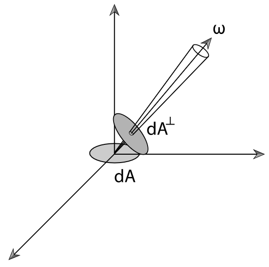
Radiance \(L\) is defined as flux per unit solid angle \(d\omega\) per unit projected area \(dA^\bot\)
In terms of irradiance, radiance measures irradiance or radiant exitance with respect to solid angles:
$$L(p,\omega)=\lim_{\Delta\omega\rightarrow 0}\frac{\Delta E_\omega(p)}{\Delta\omega} = \frac{dE_\omega(p)}{d\omega},$$
where \(E_\omega\) denotes irradiance at the surface that is perpendicular to the direction \(\omega\).
Radiometry
Incident and Exitant Radiance Functions
We make a distinction between radiance arriving at the point (e.g., due to illumination from a light source) and radiance leaving that point (e.g., due to reflection from a surface)
Incident Radiance
The incident radiance function \(L_i(p, \omega)\) describes the distribution of radiance arriving at a point as a function of position and direction
Exitant Radiance
The exitant radiance function \(L_o(p, \omega)\) gives the distribution of radiance leaving the point
Note that for both functions, \(\omega\) is oriented to point away from the surface, and, thus, for example, \(L_i(p,-\omega)\) gives the radiance arriving on the other side of the surface than the one where \(\omega\) lies
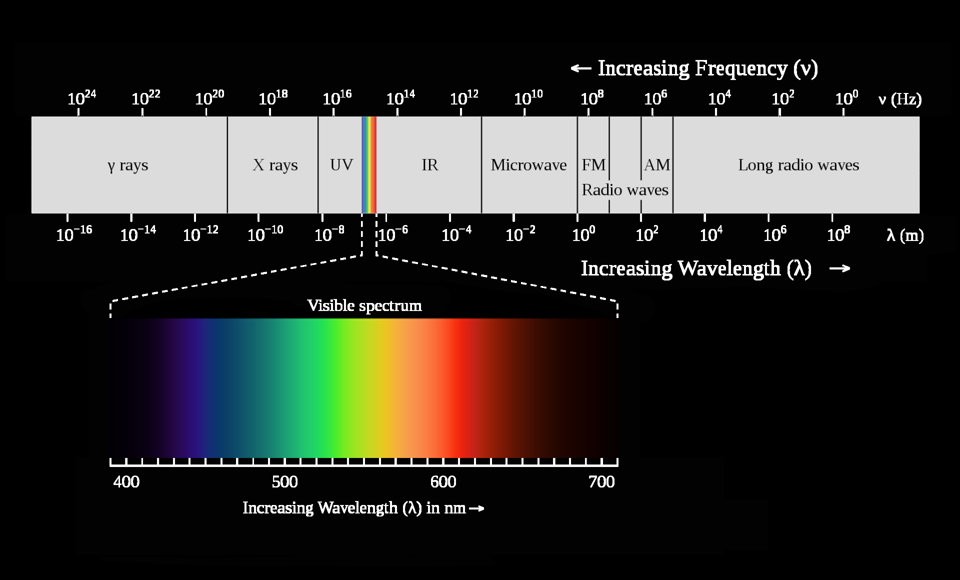
Photometry
Photometry is the study of visible electromagnetic radiation in terms of its perception by the human visual system
All of the radiometric measurements like flux, radiance, etc. have corresponding photometric measurements
Luminosity Function
Our visual system responds differently to different wavelengths
- Luminous efficiency function \(V(\lambda)\) (aka spectral response curve) describes the relative sensitivity of the human eye to various wavelengths
- Represents the average human spectral response
- Separate curves exist for light and dark adaptation of the eye
Each radiometric quantity can be converted to its corresponding photometric quantity by integrating against the luminosity function.
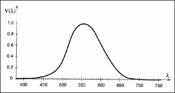
Example
Radiance \(L(\lambda)\) can be converted to luminance \(Y\) as
$$ Y = \int_\lambda L(\lambda)V(\lambda)d\lambda$$
Photometry
Photometry is the study of visible electromagnetic radiation in terms of its perception by the human visual system
All of the radiometric measurements like flux, radiance, etc. have corresponding photometric measurements
| Radiometric | Unit | Photometric | Unit | |
|---|---|---|---|---|
| Radiant energy | joule (Q) | Luminous energy | talbot (T) | |
| Radiant flux | watt (W) | Luminous flux | lumen (lm) | |
| Intensity | W / sr | Luminous flux | lm / sr = candela (cd) | |
| Irradiance | W / m^2 | Illuminance | lm / m^2 = lux (lx) | |
| Radiance | W / (m^2 sr) | Luminance | lm / (m^2 sr) = cd / m^2 = nit |
Physics-based quantities
Perception-based quantities
The Rendering Equation
The most important equation in Computer Graphics
In Physics called radiative transport equation and expresses energy equilibrium in scene:
Exitant radiance = emitted radiance + reflected radiance
Emitted radiance (\(L_e\)) describes the emissivity of the surface and is non-zero only for light sources
Reflected radiance (\(L_r\)) is in general an integral over all possible incoming directions of radiance times angle-dependent surface reflection function.
It leads to Fredholm integral equation of second kind: thus, numerical methods are necessary to compute an approximate solution
The Rendering Equation
Working with Radiometric Integrals
Example
Computation of irradiance at a point
Irradiance at a point \(p\) with surface normal \(\vec{n}\) due to radiance over a set of directions \(\Omega\) is
$$E(p,\vec{n}) = \int_\Omega L_i(p, \omega_i)\left|\cos\theta_i\right|d\omega, $$
where \(L_i(p,\omega_i)\) is the incident radiance function and the \(\cos\theta_i\) term in this integral is due to the \(dA^\bot\) term in the definition of radiance
- \(\theta_i\) is measured as the angle between \(\omega_i\) and the surface normal \(\vec{n}\)
- Irradiance is usually computed over the hemisphere \(H^2(\vec{n})\) of directions about a given surface normal \(\vec{n}\)
The Rendering Equation
Working with Radiometric Integrals
Integrals over Spherical Coordinates
Computation of irradiance at a point
Irradiance at a point \(p\) with surface normal \(\vec{n}\) due to radiance over a set of directions \(\Omega\) is
$$E(p,\vec{n}) = \int_\Omega L_i(p, \omega)\left|\cos\theta\right|d\omega $$
We can thus see that the irradiance integral over the hemisphere can equivalently be written as
$$E(p,\vec{n}) = \int^{2\pi}_{0}\int^{\pi/2}_{0} L_i(p, \theta,\phi)\cos\theta \sin\theta d\theta d\phi $$
Note: if the radiance is the same from all directions, the equation simplifies to
$$E=\pi L_i$$
The Rendering Equation
Working with Radiometric Integrals
Integrals over Area
Computation of irradiance at a point
Irradiance at a point \(p\) with surface normal \(\vec{n}\) due to radiance over a set of directions \(\Omega\) is
$$E(p,\vec{n}) = \int_\Omega L_i(p, \omega)\left|\cos\theta\right|d\omega $$
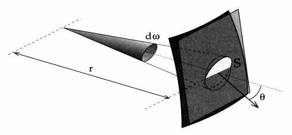
Therefore, we can write the irradiance integral for the quadrilateral source as
$$E(p,\vec{n}) = \int_S L\cos\theta_i\frac{\cos\theta_o}{r^2}dS $$
To compute irradiance at a point \(p\) from a quadrilateral source, it’s easier to integrate over the surface area of the source than to integrate over the irregular set of directions that it subtends. Thus \(L\) here is the emitted radiance from the surface of the quadrilateral source.
The Rendering Equation
We would like to know how much radiance is leaving the surface in the direction \(\omega_o\) toward the camera, \(L_o(p,\omega_o)\), as a result of incident radiance along the direction \(\omega_i\), \(L_i(p,\omega_i)\).
Because of the linearity assumption from geometric optics, the reflected differential radiance is proportional to the irradiance:
$$dL_r(p,\omega_o)\propto dE(p,\omega_i)$$
or
$$dL_r(p,\omega_o) = k\cdot dE(p,\omega_i)$$
or
$$dL_r(p,\omega_o) = f_r(p,\omega_o,\omega_i)\cdot dE(p,\omega_i)$$
Recall: Irradiance at a point \(p\) with surface normal \(\vec{n}\) due to radiance over a set of directions \(\Omega\) is
$$E(p,\omega_i) = \int_\Omega L_i(p, \omega_i)\left|\cos\theta_i\right|d\omega $$
The Rendering Equation
We would like to know how much radiance is leaving the surface in the direction \(\omega_o\) toward the camera, \(L_o(p,\omega_o)\), as a result of incident radiance along the direction \(\omega_i\), \(L_i(p,\omega_i)\).
Because of the linearity assumption from geometric optics, the reflected differential radiance is proportional to the irradiance:
$$dL_r(p,\omega_o)=f_r(p,\omega_o,\omega_i) L_i(p,\omega_i)\cos\theta_id\omega$$
Recall: Irradiance at a point \(p\) with surface normal \(\vec{n}\) due to radiance over a set of directions \(\Omega\) is
$$E(p,\omega_i) = \int_\Omega L_i(p, \omega_i)\left|\cos\theta_i\right|d\omega $$
The rendering Equation:
$$ L_o(p,\omega_o) = L_e(p,\omega_o) + \int_{H^2(\vec{n})} f_r(p,\omega_o,\omega_i)L_i(p,\omega_i)\cos\theta_i d\omega_i$$
The Rendering Equation
The bidirectional reflectance distribution function (BRDF) gives a formalism for describing reflection from a surface
$$ f_r(p,\omega_o,\omega_i) = \frac{dL_o(p,\omega_o)}{dE(p,\omega_i)}$$
BRDF
BRDF
is the key term of the rendering equation
BRDF
is the core of every software shader class
The Rendering Equation
The bidirectional reflectance distribution function (BRDF) gives a formalism for describing reflection from a surface
$$ f_r(p,\omega_o,\omega_i) = \frac{dL_o(p,\omega_o)}{dE(p,\omega_i)}$$
BRDF Properties
Reciprocity
Helmholtz reciprocity principle: BRDF remains unchanged if incident and reflected directions are interchanged
$$ f_r(p,\omega_o,\omega_i) = f_r(p,\omega_i,\omega_o) $$
Energy Conservation
The total energy of light reflected is less than or equal to the energy of incident light. For all directions \(\omega_o\)
$$ \int_{H^2(\vec{n})} f_r(p,\omega_o,\omega_i) \cos\theta_i d\omega_i \le 1$$
BRDF Measurement
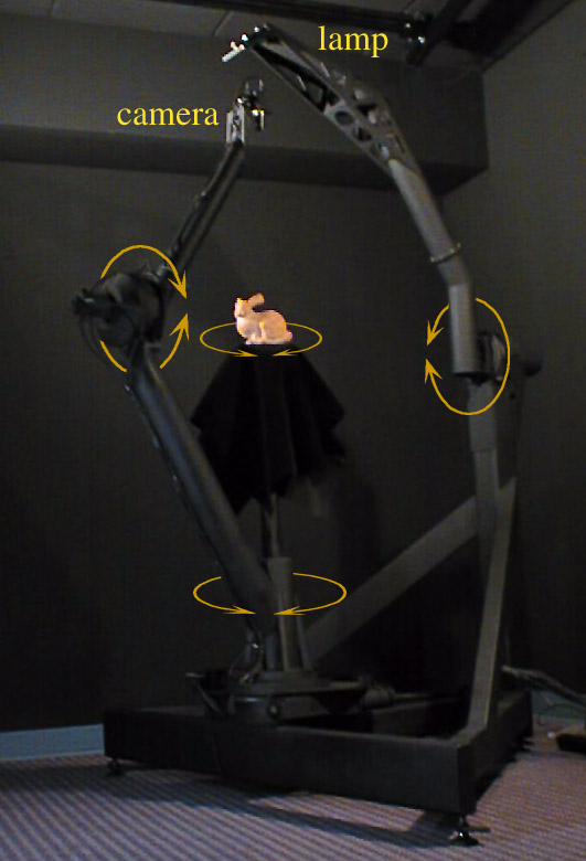
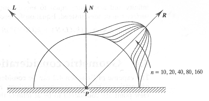
A device to measure BRDF is called Gonioreflectometer
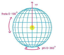
- Point light source position \((\theta_i,\phi_i)\)
- Light detector position \((\theta_o,\phi_o)\)
4 directional degrees of freedom
BRDF representation
- \(m\) incident direction samples \((\theta_i,\phi_i)\)
- \(n\) outgoing direction samples \((\theta_o,\phi_o)\)
- \(m\times n\) reflectance values (large!!!)
Rendering from Measured BRDF
Linearity, superposition principle
- Complex illumination: integrating light distribution against BRDF
- Sampled BRDF: superimposed point light sources
Interpolation
- Look-up during rendering
- Sampled BRDF must be filtered
BRDF Modeling
- Fit parameterised BRDF model to measured data
- Continuous function
- No interpolation
- Fast evaluation

BRDF of various materials
Reflectance may vary with
- Illumination angle
- Viewing angle
- Wavelength
- Polarisation
- ...
Variations due to
- Absorption
- Surface micro-geometry
- Index of refraction / dielectric constant
- Scattering
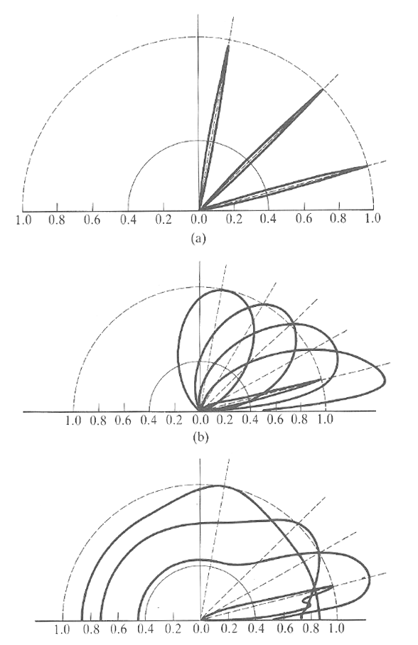
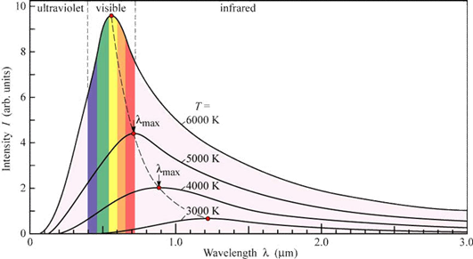
Aluminium; \(\lambda=2.0\mu m\)
Aluminium; \(\lambda=0.5\mu m\)
Magnesium; \(\lambda=0.5\mu m\)
BRDF Approximation
In case when BRDF measurement is impossible, an approximated model may be used
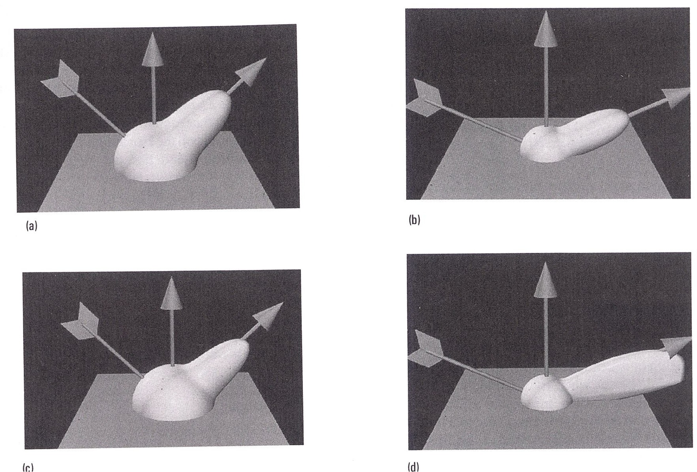
Three elemental components that can be used to model a variety of light-surface interactions
Mirror
- Reflection law
- Ideal specular reflection
Diffuse
- Lambert's law
- Ideal diffuse reflection
- Matte surfaces
Glossy
- Directional diffuse
- Shiny surfaces
BRDF
BRDF Approximation
Ideal Diffuse Reflection
Light equally likely to be reflected in any output direction (independent of input direction)
Constant BRDF
$$f_r(p,\omega_o,\omega_i)=k_d=const$$
Rendering Equation
$$L_{r,d}(p,\omega_o) = \int_{H^2(\vec{n})} k_dL_i(p,\cdot)\cos\theta_i d\omega_i = k_d L_i\cos\theta_i\int_{H^2(\vec{n})} d\omega_i = 2\pi k_d L_i \cos\theta_i \propto k_dL_i(\vec{n}\cdot\vec{I})$$
BRDF Approximation
Lambertian Diffuse Reflection
Light equally likely to be reflected in any output direction (independent of input direction)
Constant BRDF
$$f_r(p,\omega_o,\omega_i)=k_d=const$$
Rendering Equation
$$L_{r,d}(p,\omega_o) = k_dL_i(\vec{n}\cdot\vec{I})$$
Self-Luminous spherical Lambertian Light Source
$$E\propto L_o\cdot d\omega$$
Eyelight Illuminated Spherical Lambertian Reflector
$$E\propto L_o\cdot\cos\theta\cdot d\omega$$
Lambertian Objects
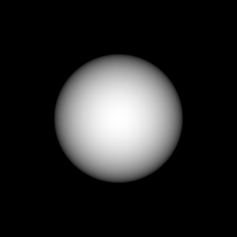
CShaderFlatCShaderEyelightThe Sun
-
Absorption in photosphere
-
Path length through photosphere longer from the Sun’s rim
The Moon
-
Surface covered with fine dust
-
Dust on TV visible best from slanted viewing angle
Lambertian Objects
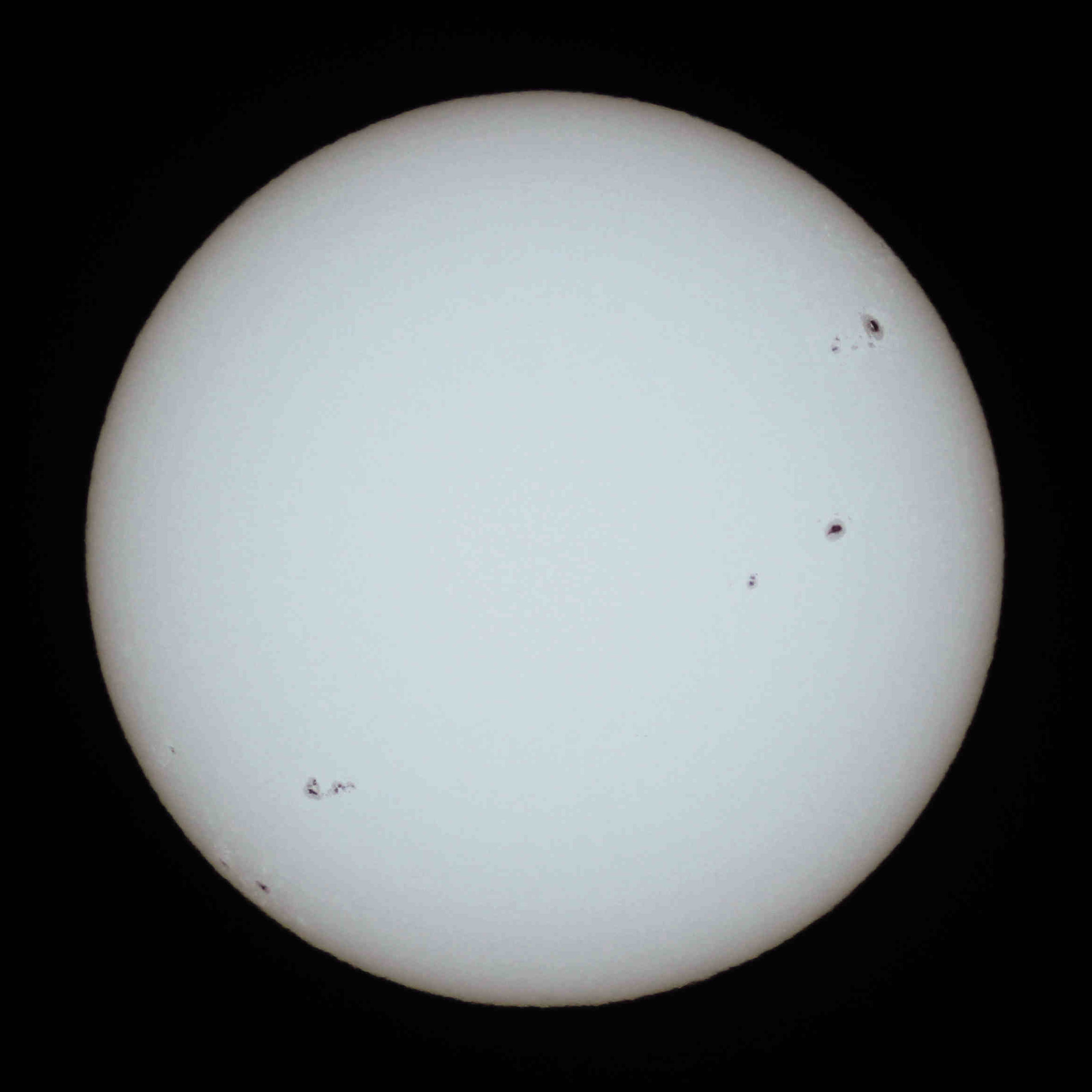
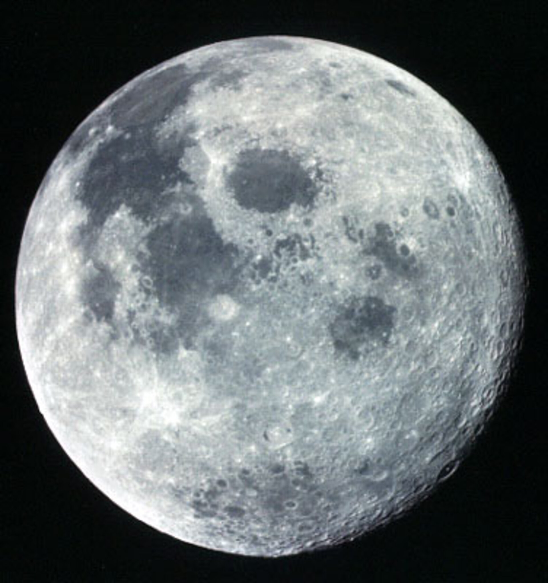
Neither the Sun nor the Moon are Lambertian
Lambertian Objects
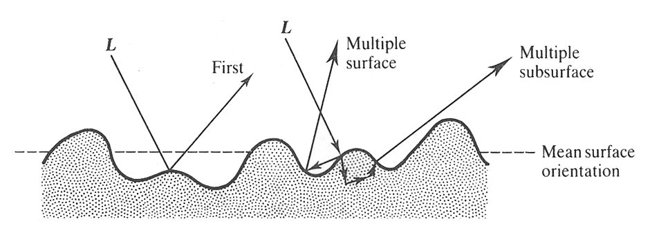
Theoretical explanation
Multiple scattering
Experimental realisation
Pressed magnesium oxide powder
Almost never valid at high angles of incidence
Paint manufacturers attempt to create ideal diffuse paints
BRDF Approximation
Ideal Specular Reflection
Angle of reflectance \(\theta_o\) is equal to angle of incidence \(\theta_i\)
Auxiliary Variables:
Reflected Ray:
BRDF Approximation
Ideal Specular Reflection
Angle of reflectance \(\theta_o\) is equal to angle of incidence \(\theta_i\)
Reflected Ray:
Reflected Ray:
BRDF Approximation
Ideal Specular Reflection
Dirac delta function \(\delta(x)\) equal to zero everywhere except at \(x=0\)
Mirror BRDF
$$f_r(p,\omega_o,\omega_i)=\frac{\delta(\cos\theta_i-\cos\theta_o)}{\cos\theta_i}\cdot\delta(\phi_i-\phi_o\pm\pi)$$
Rendering Equation
$$L_{r,m}(p,\omega_o) = \int_{H^2(\vec{n})} \frac{\delta(\cos\theta_i-\cos\theta_o)}{\cos\theta_i}\delta(\phi_i-\phi_o\pm\pi)L_i(p,\theta_i,\phi_i)\cos\theta_i d\omega_i = L_i(p,\theta_o,\phi_o\pm\pi)$$
side view
top view
BRDF Approximation
Directional Diffuse Reflection
(Glossy Reflection)

BRDF Approximation
Directional Diffuse Reflection
(Glossy Reflection)
Glossy reflection appears due to surface roughness
Empirical models
Physical models
BRDF Approximation
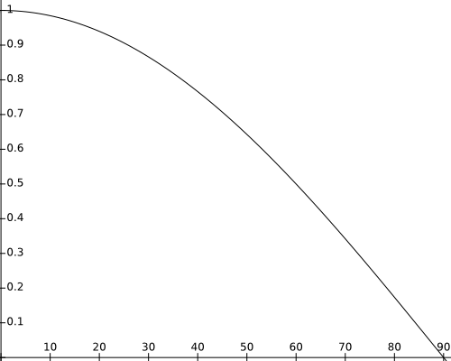
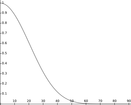
Phong
BRDF
$$f_r(p,\omega_o,\omega_i)=k_s\cos\theta^{k_e}_{\vec{r}\vec{v}}=k_s\left(\vec{r}\cdot\vec{v} \right)^{k_e}$$
Rendering Equation
$$L_{r,s}(p,\omega_o) = k_sL_i\left(\vec{r}\cdot\vec{v}\right)^{k_e}$$
BRDF Approximation
Phong
Rendering Equation
$$L_{r,s}(p,\omega_o) = k_sL_i\left(\vec{r}\cdot\vec{v}\right)^{k_e}$$

BRDF Approximation
Blinn-Phong
Make use of a halfway vector \(\vec{h}=(\vec{I}+\vec{v})/|\vec{I}+\vec{v}|\) in order to approximate Phong reflectiion model.
BRDF
$$f_r(p,\omega_o,\omega_i)=k_s\cos\theta^{k_e}_{\vec{h}\vec{n}}=k_s\left(\vec{h}\cdot\vec{n} \right)^{k_e}$$
Rendering Equation
$$L_{r,s}(p,\omega_o) = k_sL_i\left(\vec{h}\cdot\vec{n}\right)^{k_e}$$
BRDF Approximation
Wrap-up
We have considered 3 elemental components that can be used to model a variety of light-surface interactions
Mirror \(L_{r,m}\)
Diffuse \(L_{r,d}\)
Glossy \(L_{r,s}\)
BRDF
Which can be also extended with more terms
Ambient \(L_{r,a}\)
(approximate indirect illumination)
Perfect Transmission \(L_{r,t}\)
(only possible with recursive raytracing)
BRDF Approximation
Phong
$$L_r=k_aL_{i,a}+k_d\sum_lL_i(\vec{I}_l\cdot\vec{n})+k_s\sum_lL_i(\vec{r}(\vec{I}_l)\cdot\vec{v})^{k_e}$$
Blinn-Phong
$$L_r=k_aL_{i,a}+k_d\sum_lL_i(\vec{I}_l\cdot\vec{n})+k_s\sum_lL_i(\vec{h}\cdot\vec{n})^{k_e}$$
Here index \(l\) represents point light sources and the color of specular reflection equals to the light source
Both Phong and Blinn-Phong reflection models are empirical (heuristic) models
- Contradict physics
- Purely local illumination
- Only direct light from the light sources
- No further reflection on other surfaces
- Constant ambient term
- Often light sources and viewer assumed to be far away
BRDF Approximation
Microfacet Model
Idea
- Rough surfaces can be modelled as a collection of small microfacets
- The distribution of faces may be described statistically
Microfacet surface models are often described by a function that gives the distribution of microfacet normals with respect to the surface normal
The greater the variation of microfacet normals, the rougher the surface is
Smooth surfaces have relatively little variation of microfacet normals
BRDF Approximation
Microfacet Model
Important geometric effects to consider with microfacet reflection models:
Inter-reflection
Light bounces among the microfacets before reaching the viewer
Shadowing
Analogously, light does not reach the microfacet
Masking
The microfacet of interest is not visible to the viewer due to occlusion by another microfacet
BRDF Approximation
Torrance-Sparrow
Idea:
For directions \(\omega_i\) and \(\omega_o\), only microfacets with normal \(\omega_h\) reflect light (i.e. \(\vec{n}_f\equiv\vec{h}\))
BRDF
$$f_r(p,\omega_o,\omega_i)=\frac{D(\omega_h)G(\omega_i, \omega_o)F_r(\omega_o)}{4\cos\theta_i\cos\theta_i}$$
-
\(D(\omega_h)\): statistical microfacet distribution function, that gives the probability that a microfacet has orientation \(\omega_h\)
-
\(G(\omega_i, \omega_o)\): geometric attenuation term, which describes the fraction of microfacets that are masked or shadowed
- \(F_r(\omega_o)\): Fresnel term, computed by Fresnel equation and relates incident light to reflected light for each planar microfacet
BRDF Approximation
Torrance-Sparrow
Statistical microfacet distribution function
As an approximation we may assume isotropic microfacet distributions: \(D(\omega_h)\equiv D(\theta_h)\), where \(\theta_h=\vec{n}\cdot\vec{h}\)
BRDF
$$f_r(p,\omega_o,\omega_i)=\frac{D(\omega_h)G(\omega_i, \omega_o)F_r(\omega_o)}{4\cos\theta_i\cos\theta_i}$$
Blinn: $$ D(\theta_h)=\frac{e+2}{2\pi}\cos^e\theta_h $$
Torrance - Sparrow:
$$D(\theta_h)=e^{-\left(\frac{\theta_h}{\sqrt{2}\alpha}\right)^2}$$
Beckmann - Spizzichino:
$$D(\theta_h)=\frac{1}{4\sigma^2\cos^4\theta_h}e^{-\tan^2\theta_h/\sigma^2}$$
BRDF Approximation
Torrance-Sparrow
Geometric Attenuation Factor
Fully illuminated and visible: $$ G(\omega_i,\omega_o)=1 $$
Partial masking of reflected light:
$$G(\omega_i,\omega_o)=\frac{2\cos\theta_h\cos\theta_o}{(\vec{v}\cdot\vec{h})}$$
Partial shadowing of incident light:
$$G(\omega_i,\omega_o)=\frac{2\cos\theta_h\cos\theta_i}{(\vec{v}\cdot\vec{h})}$$
The resulting geometric attenuation factor:
$$G(\omega_i,\omega_o)=\min\left(1,\frac{2(\vec{n}\cdot\vec{h})(\vec{n}\cdot\vec{v})}{(\vec{v}\cdot\vec{h})},\frac{2(\vec{n}\cdot\vec{h})(\vec{n}\cdot\vec{I})}{(\vec{v}\cdot\vec{h})}\right)$$
BRDF Approximation
Phong VS Torrance-Sparrow
Phong:
Torrance-Sparrow:
Radiation characteristics
Directional light
- Spot-lights
- Projectors
- Distant sources
Diffuse emitters
- Torchieres
- Frosted glass lamps
Ambient light
- “Photons everywhere”
Emitting area
Volume
- Neon advertisements
- Sodium vapor lamps
Area
- CRT, LCD display
- (Overcast) sky
Line
- Clear light bulb, filament
“Point”
- Xenon lamp
- Arc lamp
- Laser diode
Light Sources
Light Source Classification
Power (total flux)
- Emitted energy / time
Active emission size
- Point, line, area, volume
Spectral distribution
- Thermal, line spectrum
Directional distribution
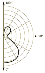
- Goniometric diagram
Light Sources
Light Source Specifications
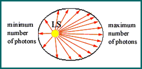
Point light with isotropic radiance
Power (total flux) of a point light source
$$\Phi$$
Light Sources
Point Light Source
Intensity of a light source (radiance cannot be defined, no area)
$$I=\frac{\Phi}{4\pi}$$
Irradiance on a sphere with radius \(r\) around light source:
$$E=\frac{\Phi}{4\pi r^2}$$
Irradiance on some other surface \(S\)
$$E(p)=\frac{d\Phi}{dS}=I\frac{d\omega}{dS}=\frac{\Phi}{4\pi}\frac{dS\cos\theta}{r^2dS}=\frac{\Phi\cos\theta}{4\pi r^2}$$
Irradiance \(E\): power per \(m^2\)
- Illuminating quantity
Distance-dependent
- Double distance from emitter: area of sphere is four times bigger
Irradiance falls off with inverse of squared distance
- Only for point light sources
Light Sources
Point Light Source
Inverse Square Law
Flux from a point light source measured by the total amount of energy passing through imaginary spheres around the light