Lesson 4:
Spatial Index Structures
Contents
- Introduction
- Bounding Volumes
- Space Partitioning with Half-Spaces
Introduction
Ray-Geometry Intersection
bool CScene::intersect(Ray& ray) const
{
  bool hit = false;
  for (auto& pPrim : m_vpPrims)	   // iterate over all the primitives
    hit |= pPrim->intersect(ray);  // check intersection
  return hit;
}std::vector<std::shared_ptr<IPrim>> m_vpPrims; // All scene primitivesTraversing all primitives in the scene for each ray is inefficient!
Need auxiliary spatial index structures to accelerate this process
Partition the space
- Flat: Uniform Grid, hierarchies of grids
- Hierarchical: Octree, Binary Space Partition (BSP), Kd-Tree
Partition the objects
- Flat: Bounding Volumes
- Hierarchical: Bounding Volume Hierarchies (BVH)
Spatial Index Structures for Ray Tracing
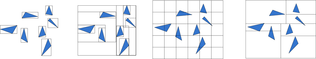
Bounding Volumes
BVH
Uniform Grid
Kd-Tree
Note: Bounding Volumes are used in all presented techniques as they are needed to define each primitive to the corresponding cell of an acceleration structure
How to evaluate an acceleration structure?
How fast is it to construct the structure?
- Building a hierarchy for n primitives takes O(n log n) time
- Inserting n primitives into a uniform grid takes O(n) time
How much memory will it use?
- A tree for n primitives takes O(n) space
- A uniform grid subdividing the space takes O(nx∗ny∗nz) space
How fast is it for a ray to traverse in the structure?
- Root to Leaf traversal is O(log n)
- Need (efficient) methods for finding neighbors in both hierarchies and flat data structures
Bounding Volumes
Idea:
Enclose each primitive with a simpler piece of geometry
E.g. sphere or box (axis-aligned, object-aligned)
A ray may hit enclosed primitive only if it hits the bounding volume first
Avoid expensive intersection test with the object
Commonly used Bounding Volumes:
Sphere
- Very fast intersection computation
- Often inefficient because too large
Axis-aligned bounding box (AABB)
- Very simple intersection computation (min-max)
- Sometimes too large
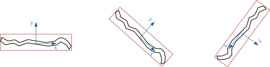
Oriented bounding-box (OBB)
- Often better fit
- Fairly complex computation
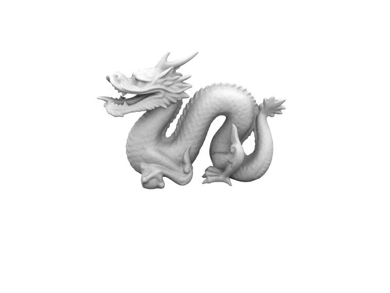
Bounding Sphere
- A sphere enclosing all of the vertices of the object
- Fastest bounding volume for intersection test with a ray
- Minimise the radius of the bounding sphere
- For a triangle or a tetrahedron, the minimal radius is simply the radius of its circumsphere
- How about more complicated geometry?
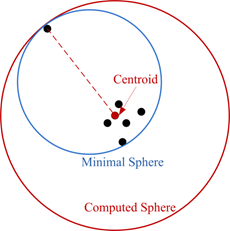
An intuitive way:
- Compute the centroid \( \vec{P}_c \) of all vertices
- Loop through all vertices and compute the maximal \( | \vec{P}_i-\vec{P}_c |^2 \) to find the farthest vertex \( \vec{P}_{farthest} \) from \( \vec{P}_c \)
- Return \( |\vec{P}_{farthest}-\vec{P}_c |^2 \) as the minimal radius
- A counter example: a crowd of points with one discrete point far away, the radius calculated in this way is about twice as big as the minimal one
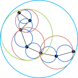
A hierarchical way:
- Build the bounding sphere for each triangle
- Recursively merge the neighbouring spheres into a larger one until all the spheres are merged into one sphere
- Return the radius of that sphere as the minimal radius
Optimal methods:
- Randomized Linear programming, running in expected O(n) time.
Constructing Bounding Sphere
Advantages:
-
Constructing a bounding sphere is fast
-
Ray-sphere intersection test is easy
-
No need to change when object rotates
Disadvantages:
-
Cannot tightly enclose the object in some cases, e.g., long and thin objects, which leads to false positives
Pros & Cons of Bounding Sphere
... is trivial:
-
Loop through all of the vertices and find the min and max values in each dimension separately
-
Use the min / max values as the bottom-left / top-right corners of the bounding box
Constructing AABB
Ray-Box Intersection
A box is the intersection of 3 pairs of slabs in 3 dimensions
- Each slab contains two parallel planes and the space between them
We can detect the intersection between the ray and the box by detecting the intersections between the ray and the three pairs of slabs
- For each pair of slabs there are two intersection points tnear and tfar, and there are 6 intersection points in total for 3 pairs
- If the maximal tnear is ahead of the minimal tfar on the ray, the ray misses the box. Otherwise it hits the box.
Bounded Volume
Bounded Volume
Ray-Box Intersection
Bounded Volume
Bounded Volume
bool intersect(Ray& ray) {
    calculate tnear.x , tfar.x , tnear.y , tfar.y , tnear.z , tfar.z on 3 axes;
    tnear = max(tnear.x , tnear.y , tnear.z);
    tfar  = min(tfar.x , tfar.y , tfar.z);
    if (tnear < tfar && tnear < ray.t) {
        ray.t = tnear;    // report intersection at tnear
        return true;
    }
    return false;         // no intersection
}
Advantages:
-
Constructing an AABB is simple
-
Simply scan over all vertices and find min and max values in each dimension in O(n) time
-
-
Ray-box intersection test is fast
Disadvantages:
-
Need to recalculate the bounding box any time an object rotates (unless the ray is transformed into object space)
-
Cannot tightly enclose the object (similar to spheres)
Pros & Cons of AABB
The orientation of the box depends on the orientation of the object:
-
Don’t need to recompute the box when an object rotates
-
Can pre-compute OBB in object space and transform OBB to world space with the object (same is true for spheres)
How to compute the orientation of the object?
-
Singular Value Decomposition
-
Compute the covariance matrix and the eigenvalues and the corresponding eigenvectors of the 3x3 matrix
-
Using these eigenvectors as the basis of the local coordinate system of the bounding box
Constructing OBB
for a Triangle Primitive
Compute the mean centroid of all triangles:
$$ \vec{\mu}=\frac{1}{n}\sum^{n}_{i=0}\frac{\vec{a}_i+\vec{b}_i+\vec{c}_i}{3}, $$ where \( \vec{a}_i \), \( \vec{b}_i \) and \( \vec{c}_i \) are the vertices if ith triangle, and \( n \) is the number of triangles.
Construct the \( 3\times 3 \) covariance matrix \( C \):
the element \( c_{jk} \) is computed as:
$$ c_{jk} = \frac{1}{3n}\sum^{n}_{i=0}\left(\hat{\vec{a}}^{j}_{i}\hat{\vec{a}}^{k}_{i} + \hat{\vec{b}}^{j}_{i}\hat{\vec{b}}^{k}_{i} + \hat{\vec{c}}^{j}_{i}\hat{\vec{c}}^{k}_{i} \right), $$
where \( \hat{\vec{a}}_i=\vec{a}_i - \vec{\mu} \) and \( \hat{\vec{a}}_i=\left( \hat{a}^{1}_{i}, \hat{a}^{2}_{i}, \hat{a}^{3}_{i} \right)^\top \)
Calculate the eigenvectors \( e_1, e_2, e_3 \) of \( C \):
All of the eigenvectors are mutually orthogonal since \( C \) is symmetric, thus we can take them as the basis vectors for the local coordinate system of the OBB
Find the extreme vertices along each basis vector and resize the bounding box to bound those vertices
(similar to the AABB)
Constructing OBB
Ray-Box (Object Oriented) Intersection
Similar to Ray-AABB intersection
-
Calculate the maximum \( t_{near} \) and the minimum \( t_{far} \)
-
The planes of the slabs are not axis aligned any more
-
Recall how to compute intersection between a ray and an arbitrary plane in 3D space
Bounded Volume
Bounded Volume
Ray-AABB intersection
Ray-OBB intersection
Ray-Box (Object Oriented) Intersection
Or we can transform the ray...
... into the OBB coordinate system and perform ray-AABB intersection test
OBB
OBB
World Coordinate System
OBB Coordinate System
Advantages:
-
Fit the object tighter than AABB
Disadvantages:
-
Extra cost for ray-box intersection
-
Finding an OBB is computationally expensive (but may be done as a pre-computation)
-
Finding the minimal OBB is hard (but an approximation – such as the one we just proposed - is usually good enough)
Pros & Cons of OBB
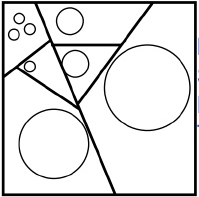
Binary Space Partition (BSP)
-
Recursively split space into halves
-
Splitting with half-spaces in arbitrary position
-
Often defined by existing polygons
-
- Generalisation of a KD Tree
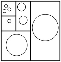
KD Tree
- Special case of BSP
- Splitting with axis-aligned half-spaces
- Defined recursively through nodes with
- Split dimension (axis index)
- Split value (1D location)
- Pointers to both children
Binary Space Partitioning
KD Tree
A binary tree for space searching
Has 2 types of nodes:
where every node is defined by its place in the overall hierarchy and described by its bounding volume
Leaf Node
-
Contains the pointer to the primitives, ascribed to that node
Branch Node
- Can be thought of as implicitly generating a splitting hyperplane that divides the space into two parts
- Points to the left of this hyperplane are represented by the left sub-tree of that node and points right of the hyperplane are represented by the right sub-tree.
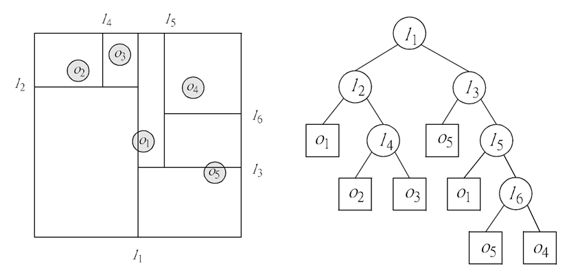
KD Tree
Implementation details
In order to implement the KD Tree we need to implement the following classes and methods:
Tree Class
-
Method to build a KD Tree using the scene primitives:
void rt::CBSPTree::build(vpPrims)
-
Method to traverse a ray:
bool rt::CBSPTree::intersect(ray)
Node Class
- Constructor to construct a leaf node:
rt::CBSPNode(vpPrims)
- Constructor to construct a branch node:
rt::CBSPNode(splitDim, splitVal, *leftNode, *rightNode)
- Auxiliary method to traverse a ray recursively:
bool rt::CBSPNode::intersect(ray, t0, t1)
where arguments t0 and t1 define ray's entering and exiting points in / out the node's bounding volume
KD Tree
Implementation details
In order to implement the KD Tree we need to implement the following classes and methods:
Bounding Box Class (AABB)
which defines bounding volume for every tree node
-
Method for checking whether a primitive belongs to the tree node or not:
bool rt::CBoundingBox::overlaps(boundingBox)
-
Method to split a bounding with a hyperplane into two halfes:
std::pair<lbox, rbox> rt::CBoundingBox::split(splitDim, splitVal)
- Auxiliary method to clip the ray entering the box, i.e. ray-aabb intersection algorith, that returns both entering and exiting points:
rt::clip(ray, &t0, &t1)
Support for AABB in every primitive
- Build and return a minimal aabb:
rt::IPrim::getBoundingBox(void)=0
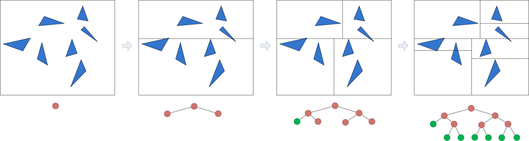
Constructing a KD Tree
In a top-down way:
- Begin with the global bounding box containing all primitives
- Choose a splitting dimension and a splitting value, subdivide the primitives on both sides of the plane into two groups and create a branch node
- When the number of primitives in each single group is below a threshold or a tree becomes too large: create a leaf node
Constructing a KD Tree
ptr_bspnode_t CBSPTree::build(const CBoundingBox& box, const std::vector<ptr_prim_t>& vpPrims, size_t depth)
{
  // Check for stoppong criteria
  if (depth > m_maxDepth || vpPrims.size() <= m_minPrimitives)
    return std::make_shared<CBSPNode>(vpPrims);                                     // Create a leaf node

  // else -> prepare for creating a branch node
  // First split the bounding volume into two halfes
  int     splitDim = MaxDim(box.getMaxPoint() - box.getMinPoint());                   // Calculate split dimension as the dimension where the aabb is the widest
  float   splitVal = (box.getMinPoint()[splitDim] + box.getMaxPoint()[splitDim]) / 2; // Split the aabb exactly in two halfes
  auto    splitBoxes = box.split(splitDim, splitVal);
  CBoundingBox& lBox = splitBoxes.first;
  CBoundingBox& rBox = splitBoxes.second;

  // Second order the primitives into new nounding boxes
  std::vector<ptr_prim_t> lPrim;
  std::vector<ptr_prim_t> rPrim;
  for (auto pPrim : vpPrims) {
    if (pPrim->getBoundingBox().overlaps(lBox))
      lPrim.push_back(pPrim);
    if (pPrim->getBoundingBox().overlaps(rBox))
      rPrim.push_back(pPrim);
  }

  // Next build recursively 2 subtrees for both halfes
  auto pLeft = build(lBox, lPrim, depth + 1);
  auto pRight = build(rBox, rPrim, depth + 1);

  // Create a branch node
  return std::make_shared<CBSPNode>(splitDim, splitVal, pLeft, pRight);
}
Ray Traversal in a KD Tree
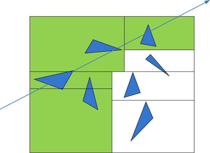
Traverse all leaf nodes in the k-d tree passed through by the ray
Ray Traversal in a KD Tree
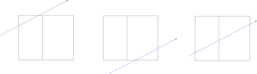
Recursive Traversal
- Each branch node has two children, there are only 3 cases for sub-node intersections:
- intersecting with the left child only
- intersecting with the right child only
- both
- The number of intersected sub-boxes and its sequence can be determined by the intersection points and faces of the ray and the node and the splitting plane of the node
Ray Traversal in a KD Tree
bool CBSPNode::intersect(Ray& ray, double t0, double t1) const
{
  if (isLeaf()) {
    for (auto& pPrim : m_vpPrims)
      pPrim->intersect(ray);
    return (ray.hit && ray.t < t1 + Epsilon);
  }
  else {
    // distnace from ray origin to the split plane of the current volume (may be negative)
    double d = (m_splitVal - ray.org[m_splitDim]) / ray.dir[m_splitDim];

    auto frontNode = (ray.dir[m_splitDim] < 0) ? Right() : Left();
    auto backNode  = (ray.dir[m_splitDim] < 0) ? Left() : Right();

    if (d <= t0) {
      // t0..t1 is totally behind d, only go to back side
      return backNode->intersect(ray, t0, t1);
    }
    else if (d >= t1) {
      // t0..t1 is totally in front of d, only go to front side
      return frontNode->intersect(ray, t0, t1);
    }
    else {
      // travese both children. front one first, back one last
      if (frontNode->intersect(ray, t0, d))
        return true;

      return backNode->intersect(ray, d, t1);
   }
}