Lesson 6
Texturing and Solids
Contents
- Introduction
- Surface Parametrisation
- Bump Mapping
- Displacement Mapping
- Environmental Mapping
- Procedural Textures
Introduction
What is Texture ?
Texture is the perceived surface quality. In CG texture is a 2D multi-channel image overlaid on the surface of a 3D solid to give it color or illusion of relief. Being the property of the geometry, textures play essential role in modeling BRDFs and thus they are managed entirely by the shaders. The quality of a textured surface is determined by the number of pixels per texture element (textel).
in OpenRT, textures are described by class rt::CTexture : public cv::Mat
Introduction
What is Texture ?
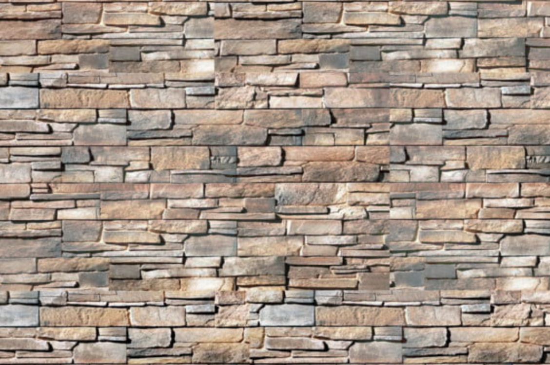
Image Texture
Image texture is a bitmap image usually stored in a common image file format. The quality of textured surface is determined by the number of pixels per telex. The resolution of image texture play a major role, which affects the overall impression of the quality of graphics in 3D-application.
Introduction
What is Texture ?
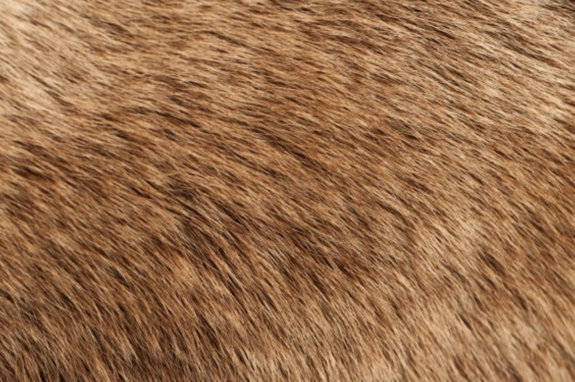
Procedural Texture
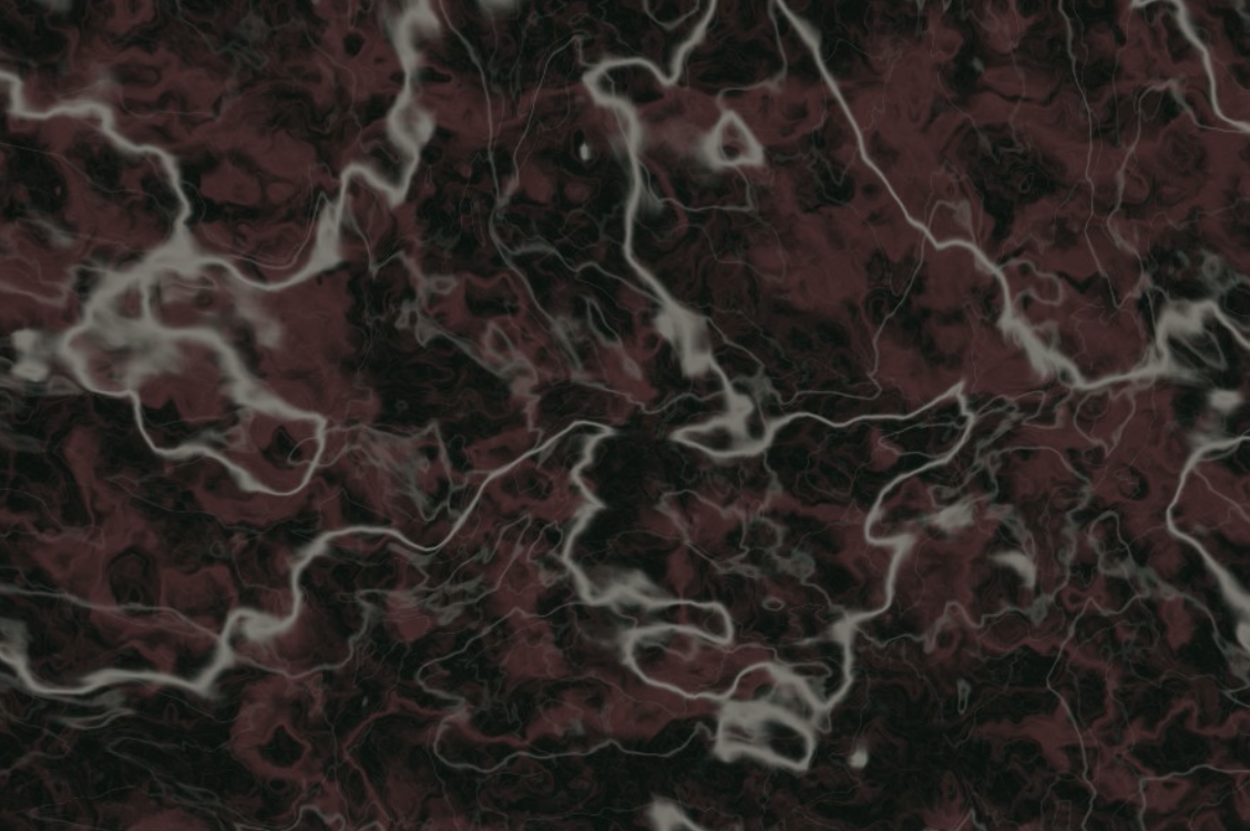
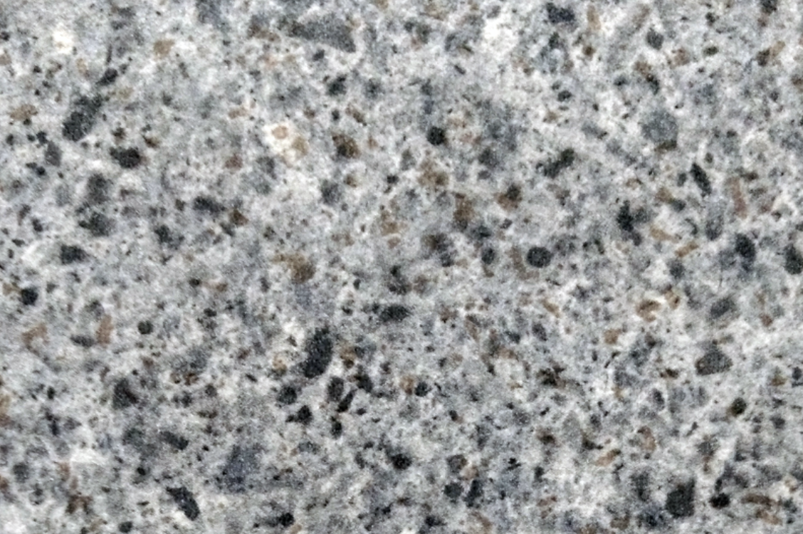
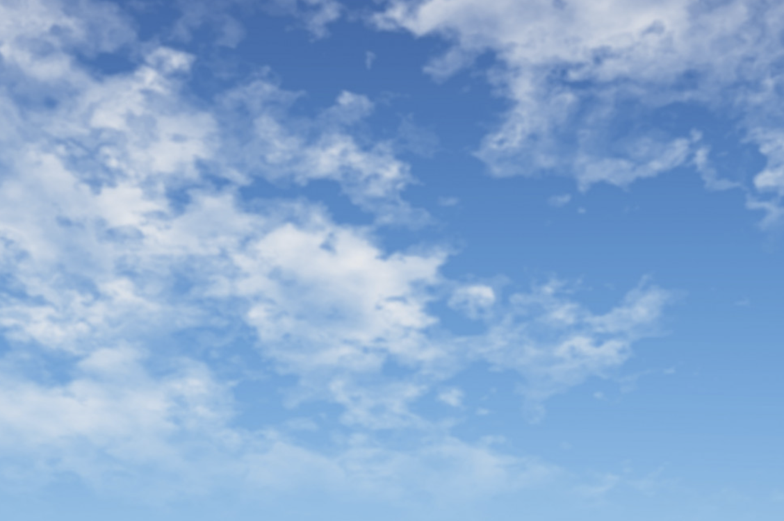
Procedural texture is created using a mathematical description (i.e. an algorithm) rather than directly stored data. The advantage of this approach is low storage cost, unlimited texture resolution and easy texture mapping. Procedural textures are used to model surface of natural elements such as clouds, marble, granite, metal, stone, and others.
Introduction
Texture-Modulated Quantities
Radiance at a point \(\vec{p}\)
- Color (RGB)
- Diffuse coefficient \(k_d\)
- Specular coefficient \(k_s\)
- Opacity \(\alpha\)
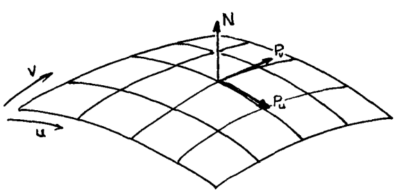
Deviation of normal vector at a point \(\vec{p}\)
Bump mapping or Normal mapping
- If vectors \(\vec{a}\) and \(\vec{b}\) are tangent to the surface at point \(\vec{p}\) and together with normal \(\vec{n}\) form an orthogonal basis, then deviate the normal by \((\Delta_1, \Delta_2)\) from the texture: \(\vec{n} = \vec{n} + \Delta_1\cdot\vec{a} + \Delta_2\cdot\vec{b} \)
Geometry Displacement
Displacement mapping
- Displace every point \(\vec{p}\) along its normal \(\vec{n}\) by the value of \(\Delta\) given in the texture:
\(\vec{p} = \vec{p} + \Delta\cdot\vec{n}\)
Distant Illumination
Environmental mapping or Reflection mapping
Introduction
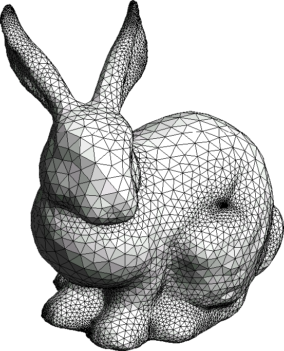
Solid is a rigid geometrical construction which consists out of multiple primitives, usually triangles. Primitives are combined into solids in order to make application of geometrical transformations and texturing easier.
in OpenRT, solids are described by class rt::CSolid
What is Solid?
Surface Parametrization
The bidirectional reflectance distribution function:
$$ f_r(\vec{p},\omega_o,\omega_i) = \frac{dL_o(\vec{p},\omega_o)}{dE(\vec{p},\omega_i)},$$
where \(\vec{p}\equiv\vec{p}(x, y, z)\) is a 3 dimentional point on solid's surface
From 3D hit-point to 2D texture coordinates
Texture is about modeling point - dependent characteristics of BRDF
Parametrization
To map a two-dimensional texture to three-dimensional surface for every 3D point \(\vec{p}(x,y,z)\) a corresponding 2D point \(\vec{q}(u,v)\) in texture must be found.
$$f:(x,y,z)\rightarrow (u,v), $$
where usually
$$u,v\in[0; 1]$$
Surface Parametrization
From 3D hit-point to 2D texture coordinates
Parametrization
To map a two-dimensional texture to three-dimensional surface for every 3D point \(\vec{p}(x,y,z)\) a corresponding 2D point \(\vec{q}(u,v)\) in texture must be found.
$$f:(x,y,z)\rightarrow (u,v), $$
where usually
$$u,v\in[0; 1]$$
When ray - primitive intersection is found, the hit-point \(\vec{p} = \vec{o} + t\cdot\vec{d}\) is encoded into the ray structure, thus parametrization can be implemented for every primitive in a method
Vec2f rt::IPrim::getTextureCoords(const Ray& ray) const = 0;Surface Parametrization
Primitive: Sphere
Cartesian to Spherical
$$r=\sqrt{x^2+y^2+z^2}$$
$$\varphi=\arctan_2\frac{y}{x}$$
$$\theta=\arccos\frac{z}{r}$$
(read more about \(\arctan_2\) function)
Spherical to Texture
Since \(\varphi\in[-\pi; \pi]\) and \(\theta\in[0;\pi]\)
$$u=\frac{\pi+\varphi}{2\pi}$$
$$v=\frac{\theta}{\pi}$$
Vec2f CPrimSphere::getTextureCoords(const Ray& ray) const
{
    Vec3f hitPoint = ray.hitPoint() - m_origin;
    float theta = acosf(hitPoint.val[1] / m_radius);	  // [0; Pif]

    float phi = atan2(hitPoint.val[2], hitPoint.val[0]);  // [-Pif; Pif]
    if (isnan(phi)) phi = 0;

    return Vec2f((Pif + phi) / (2 * Pif), theta / Pif);
}
Surface Parametrization
Primitive: Triangle
Möller-Trumbore intersection algorithm
in addition to intersection distance \(t\) implicitly calculates the barycentric intersection coordinates \((u,v)\in[0; 1]\), which may be used directly as the texel coordinates
- On construction provide additionally texture coordinates for all 3 triangle vertices
- Store barycentric coordinates in the ray structure together with \(t\) value
Vec2f CPrimTriangle::getTextureCoords(const Ray& ray) const {
    return (1.0f - ray.u - ray.v) * m_ta
           + ray.u * m_tb
           + ray.v * m_tc;
}struct Ray {
Vec3f org; // Ray origin
Vec3f dir; // Ray direction
double t; // Current/maximum hit distance
const IPrim* hit; // Pointer to currently closest primitive
float u; // Barycentric u coordinate
float v; // Barycentric v coordinate
} ray;Surface Parametrization
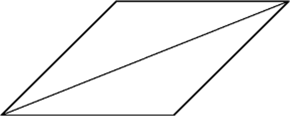
Solid: Quad
Quadrilateral Solid
Quadrilateral solid \((a,b,c,d)\) consists out of two triangles \(a,b,c)\) and \((a,c,d)\).
- On construction provide texture coordinates for all 4 quadrilateral vertices
- There is no ray-quad intersection check, only 2 ray-triangle intersection checks
Surface Parametrization
Solid: Cylinder
Cartesian to Cylindrical
$$r=\sqrt{x^2+y^2}$$
$$\varphi=\arctan_2\frac{y}{x}$$
$$h=h$$
(read more about \(\arctan_2\) function)
Spherical to Texture
Since \(\varphi\in[-\pi; \pi]\) and \(h\in[0;H]\)
$$u=\frac{\pi+\varphi}{2\pi}$$
$$v=\frac{h}{H}$$
Surface Parametrization
Solid: Cylinder
If a cylinder has \(n\) sides and every side \(s\) of a cylinder is modeled with a quad \((a,b,c,d)\), it is straightforward to calculate the 3D vertex positions as well as 2D texture coordinates:
$$u_a = \frac{s+1}{n}; v_a = 1$$
$$u_b = \frac{s}{n}; v_b = 1$$
$$u_c = \frac{s}{n}; v_c = 0$$
$$u_d = \frac{s+1}{n}; v_d = 0$$
Surface Parametrization
Complex Solids
Inverse mapping for arbitrary 3D surfaces is too complex
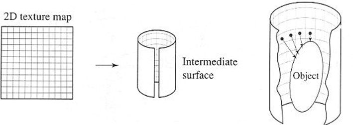
Two-Stage Texture Mapping
is an approximation technique to generate texture coordinates for every vertex of a complex-shaped solid
- Stage 1: Mapping from a texture space to a more simple intermediate 3D surface which is a reasonable approximation of the destination surface (e.g., cylinder, sphere, box or plane)
- Stage 2: Mapping from a the intermediate surface to the destination object surface
Surface Parametrization
Complex Solids
Inverse mapping for arbitrary 3D surfaces is too complex
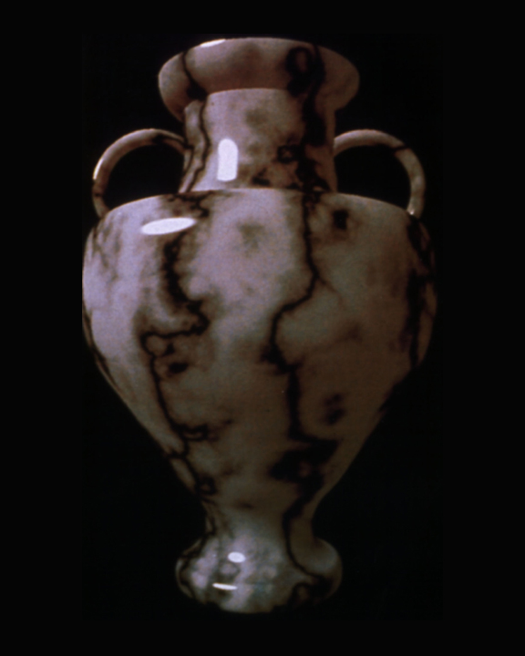
Example
Texturing a vase with different intermediate surfaces:
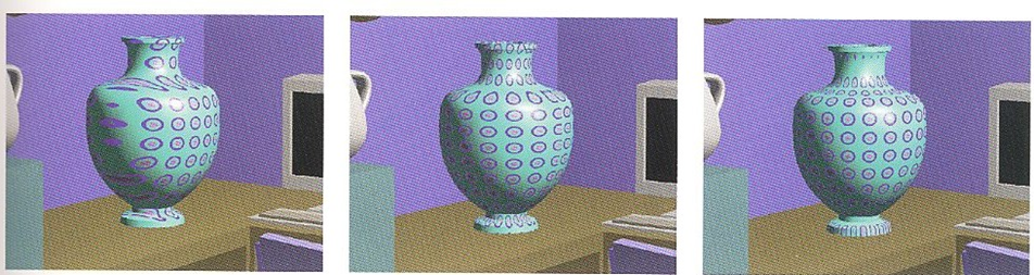
Plane
Strong distortion where object surface normal is orthogonal to the intermediate plane normal
Cylinder
Reasonably uniform mapping (symmetry!)
Sphere
Problems with concave regions
Bump Mapping / Normal Mapping
Bump Mapping
2D texture map looks unrealistically smooth across different material, especially at low viewing angle
Fool the human viewer:
- Perception of shape is determined by shading, which is determined by surface normal
- Use texture map to perturb the surface normal per fragment
- Does not actually alter the geometry of the surface
- Shade each fragment using the perturbed normal as if the surface were a different shape
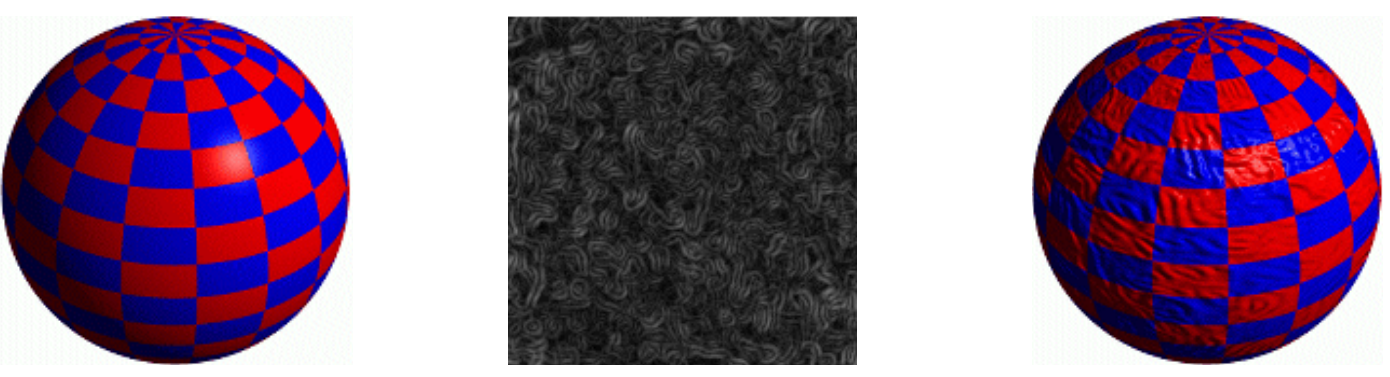
Sphere with diffuse texture
Swirly bump map
Sphere with diffuse texture and bump map
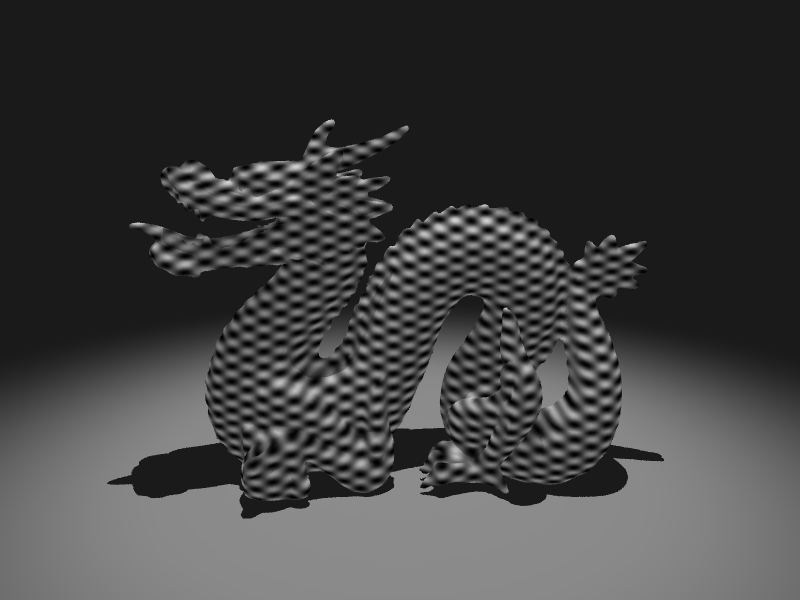
Bump Mapping
Treat the texture as a single-valued height function (height map)
- Grayscale image (CV_8UC1) stores height: black - high area; white - low (or vice versa)
- Difference in heights determines how much to perturb \(\vec{n}\) in the \((u, v)\) directions of a parametric surface
\[\frac{\partial b}{\partial u}=\frac{h_{x+1,y}-h_{x-1,y}}{dx}\]
\[\frac{\partial b}{\partial v}=\frac{h_{x,y+1}-h_{x,y-1}}{dy}\]
- compute a new, perturbed normal from \((b_u, b_v)\)
Bump Mapping
Computing Perturbed Normal
perturbed surface
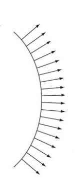
\(\vec{p}\)
\(\vec{n}\)

\(\vec{p}\)
\(\vec{p}'\)
Bump Mapping
Computing Perturbed Normal
\(\vec{p}\)
\(\vec{n}\)
\(\vec{p}\)
\(\vec{p}'\)
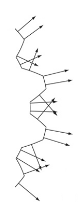
\(\vec{p}'\)
\(\vec{n}'\)
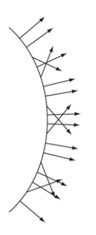
\(\vec{p}\)
\(\vec{n}'\)
Bump Mapping
Bump Mapping VS Normal Mapping
Computing \(\vec{n}’\) requires the height samples from 4 neighbours
- Each sample by itself doesn’t perturb the normal
- An all-white height map renders exactly the same as an all-black height map
Instead of encoding only the height of a point, a normal map encodes the normal of the desired surface, in the tangent space of the surface at the point
- Can be obtained from:
- a high-resolution 3D model
- photos (http://zarria.net/nrmphoto/nrmphoto.html)
- a height-map (with more complex offline computation of perturbed normals)
- filtered color texture (Photoshop, Blender, Gimp, etc. with plugin)
Bump Mapping
Bump Mapping VS Normal Mapping
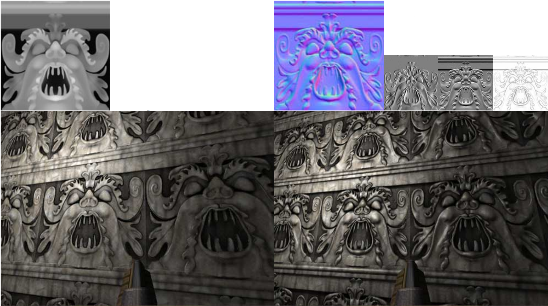
height map
normal map
\[(n_x,n_y,n_z)=(r,g,b)\]
Interpret the RGB values per texel as the perturbed normal, not height value
Displacement Mapping
Displacement Mapping
Interpret texel as offset vector to actually displace fragments:
\[\vec{p'} = \vec{p} + h(u,v)\vec{n}\]
- Correct silhouettes and shadows
-
Complex geometry at virtually no memory cost
-
Must be done during modelling stage, e.g. before ray-geometry intersection
Displacement Mapping
Interpret texel as offset vector to actually displace fragments:
\[\vec{p'} = \vec{p} + h(u,v)\vec{n}\]
- Correct silhouettes and shadows
-
Complex geometry at virtually no memory cost
-
Must be done during modelling stage, e.g. before ray-geometry intersection
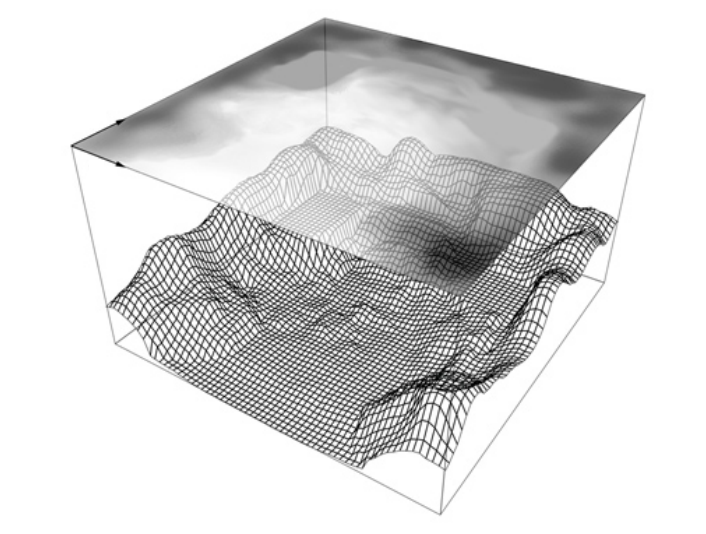
Fractal Landscapes
Procedural generation of geometry
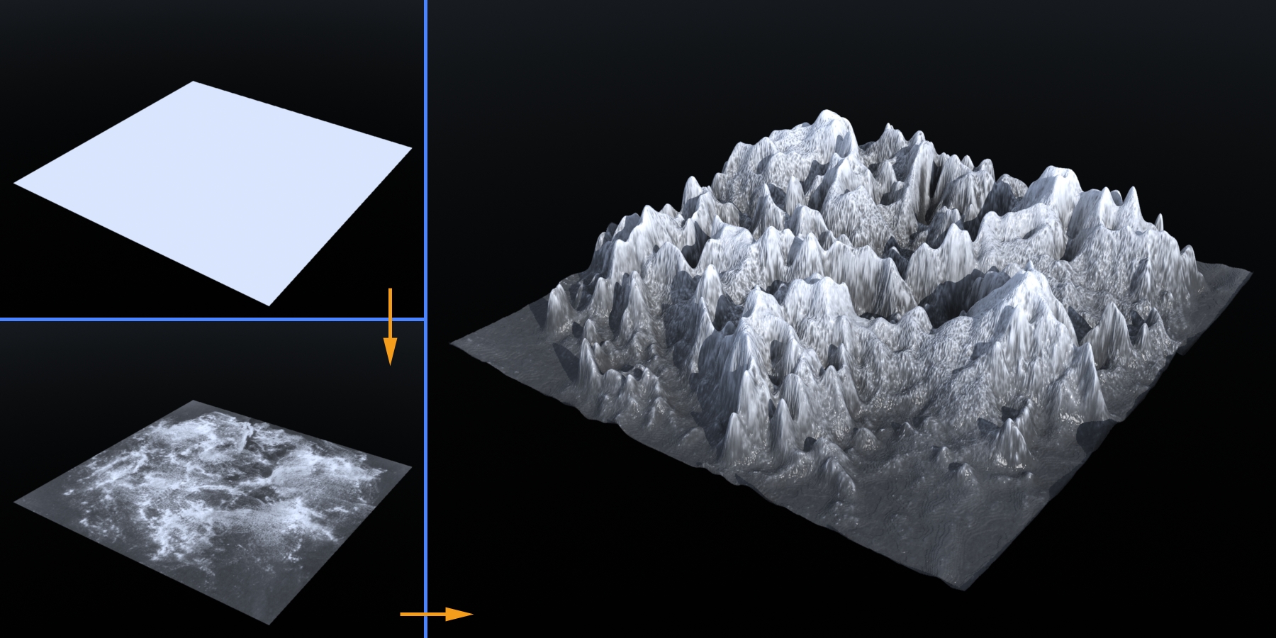
Displacement Mapping
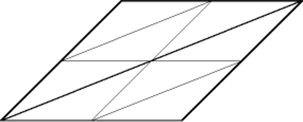
Fractal Landscapes
Coarse triangle mesh approximation
1:4 triangle subdivision
- Vertex insertion at edge-midpoints
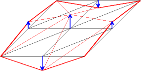
New vertex perturbation
- Displacement along normal
- Random amplitude
- Perturbation scale depends on subdivision level
- Decreasing power spectrum
- Parameter for model roughness
Recursive subdivision
- Level of detail determined by number of subdivisions

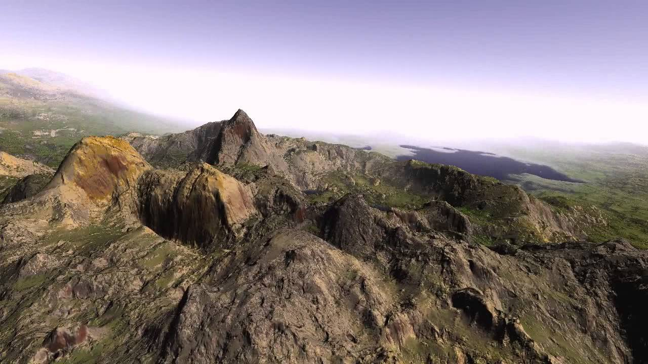
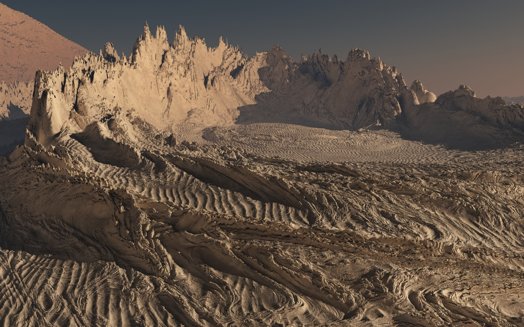
Displacement Mapping
Fractal Landscapes
Fields of Application
-
Base mesh
-
Repeated subdivision & vertex displacement
-
Water surface
-
Fog
-
…


Displacement Mapping
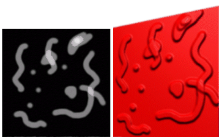
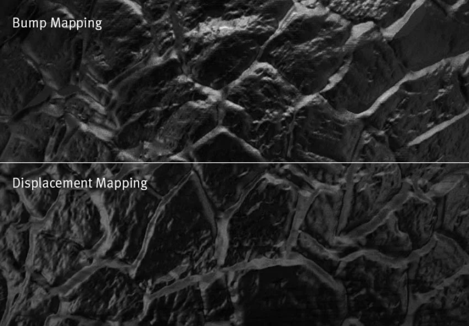
Bump Mapping VS Displacement Mapping
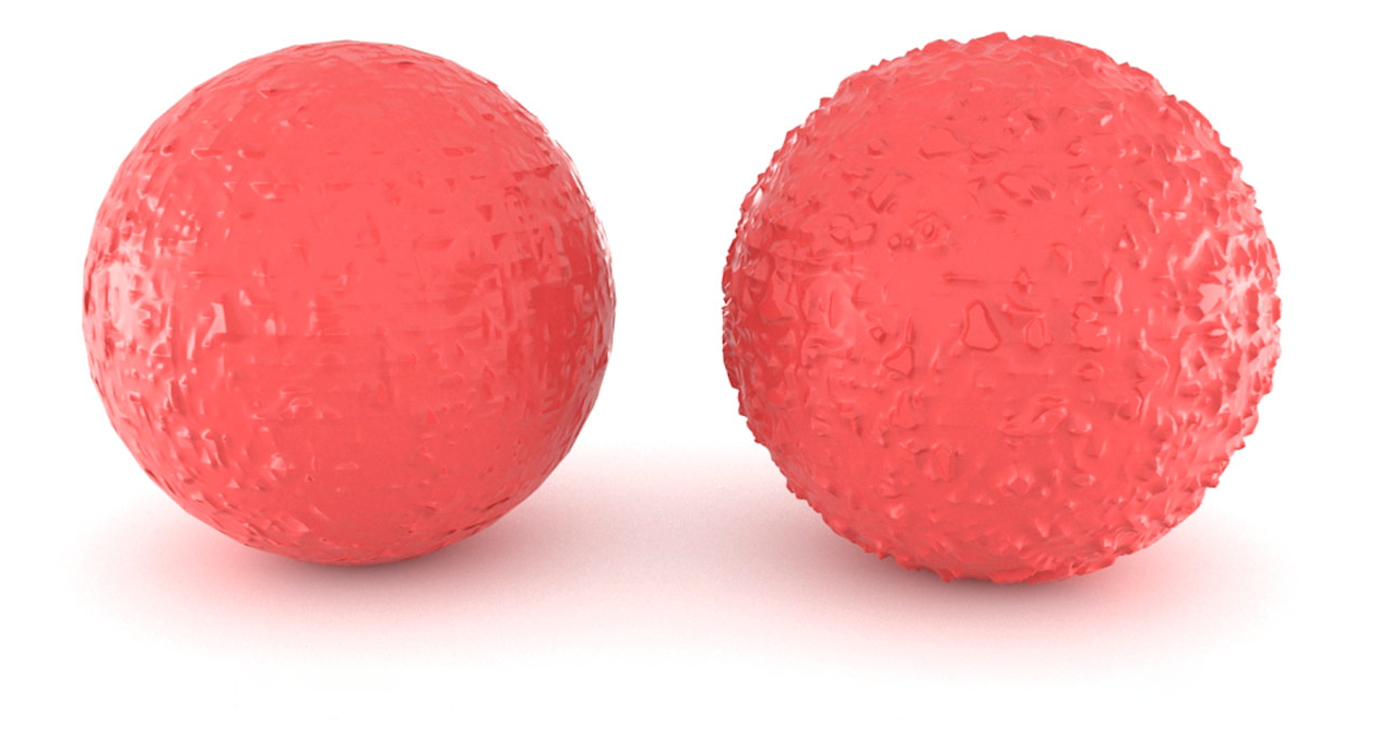
bump mapping
displacement mapping
Displacement Mapping
Bump Mapping VS Displacement Mapping

Environmental Mapping
(a.k.a Reflection Mapping)
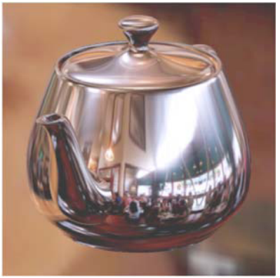
Environmental Mapping
(a.k.a Reflection Mapping)
The key to depicting a shiny-looking material is to provide something for it to reflect
- Proper reflection requires ray tracing, expensive
- Can be simulated with a pre-rendered environment, stored as a texture
- Imagine object is enclosed in an infinitely large sphere or cube
- Rays are bounced off object into environment to determine color
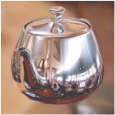
Reflection Mapping
=
Environmental Mapping
*
surface color
Environmental Mapping
Steps:
- Load environment map as a texture and apply it to environmental sphere
- Do not consider primary ray - environmental sphere intersections
- For each ray-prim intersection point \(\vec{p}\), compute normal to the prim \(\vec{n}(\vec{p})\)
- Compute the corresponding reflection vector \[\vec{r} =\vec{d}- 2\vec{n}\left(\vec{n}\cdot\vec{d}\right)\]
- Re-trace the reflection ray \(\left(\vec{p}, \vec{r}(\vec{p},\vec{n})\right)\)
- Once reflection ray hits the environmental sphere return corresponding texel from the environmental map
\(\vec{n}\)
\(\vec{p}\)
\(\vec{r}\)
primary ray
environmental sphere
omitted intersection point
really visible point
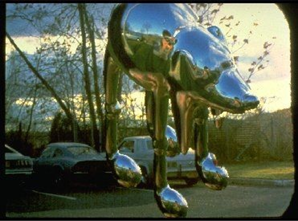
Environmental Mapping
Examples
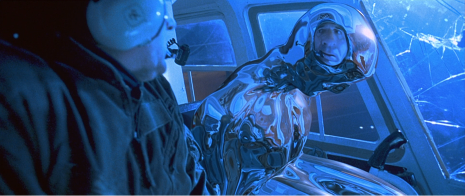
Terminator 2 motion picture 1991
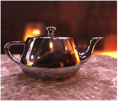
Environmental Mapping
Examples
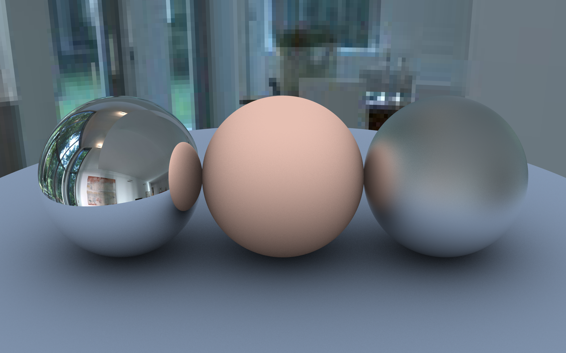
OpenRT mirror balls 2021
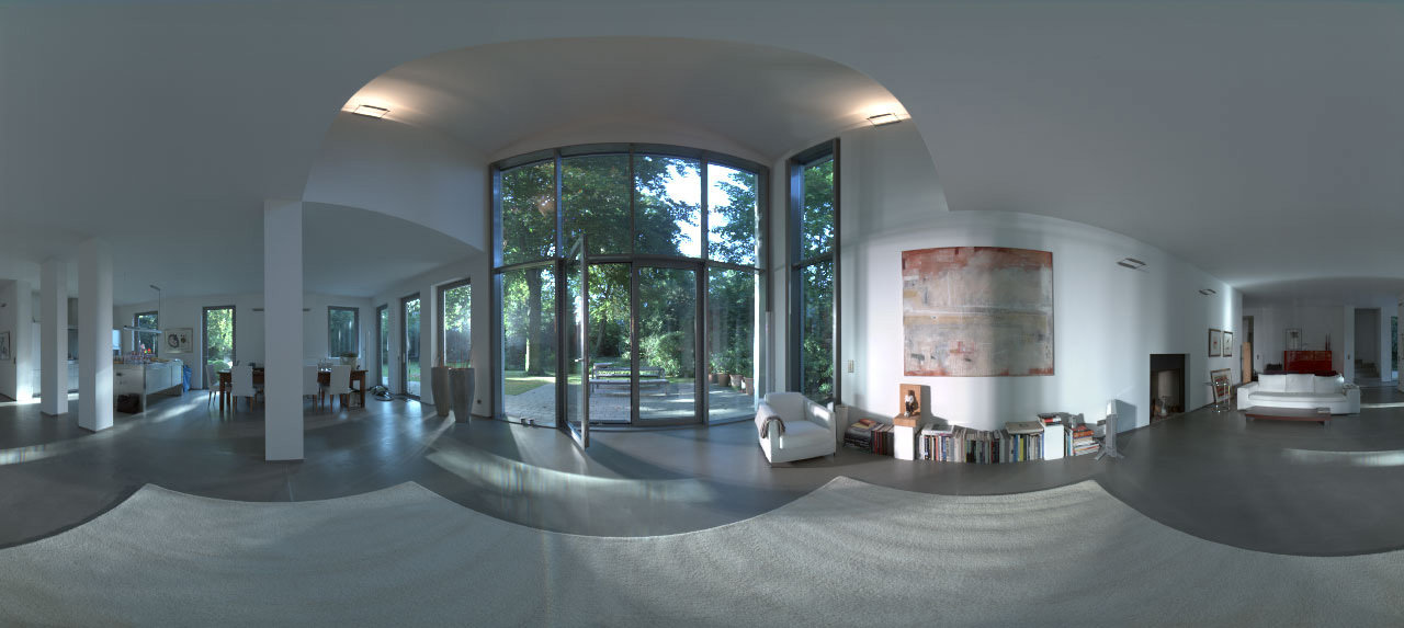
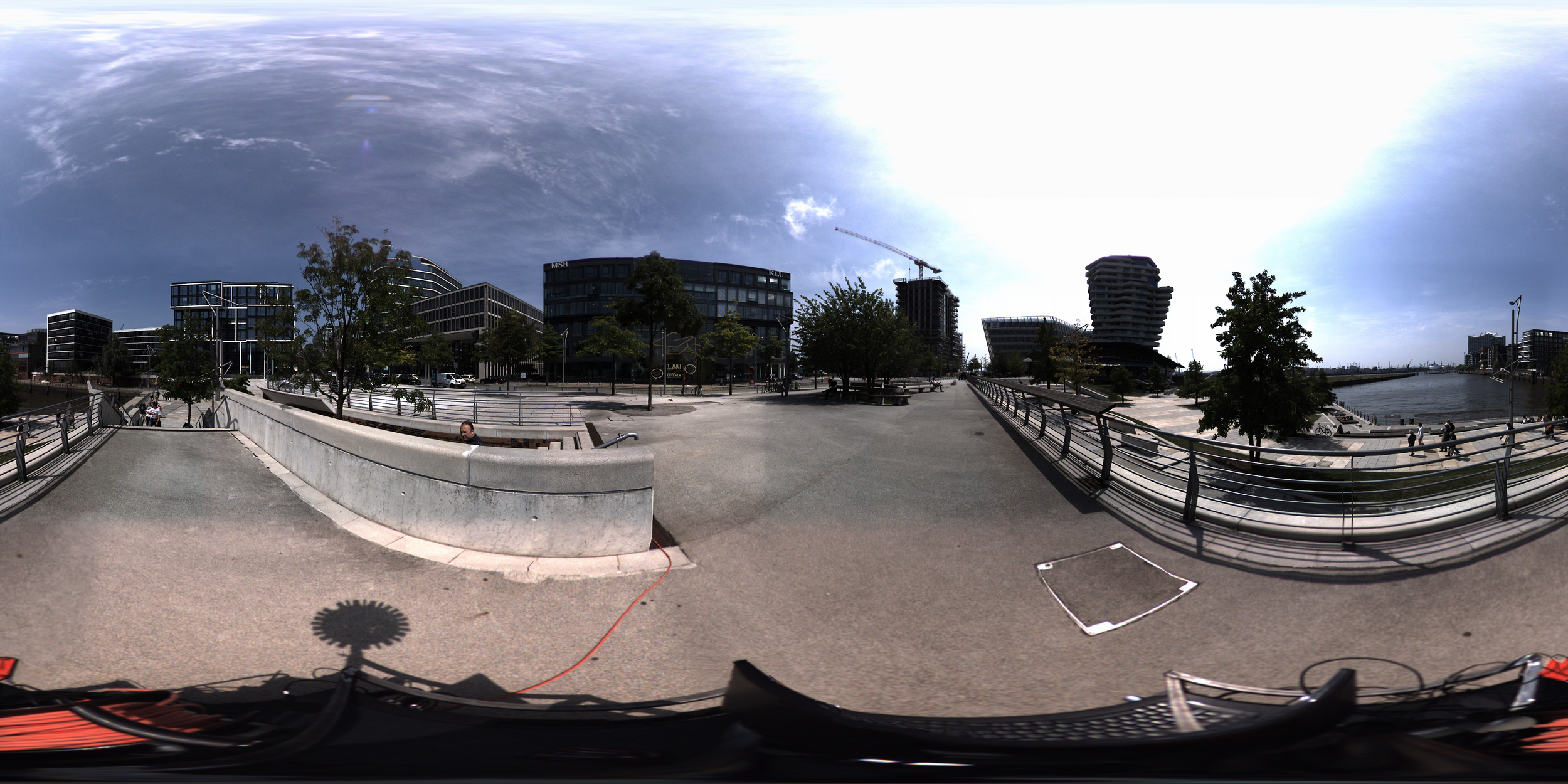
Environmental Mapping
1280 x 573 pixels size environmental map
Methods to Create Environmental Maps
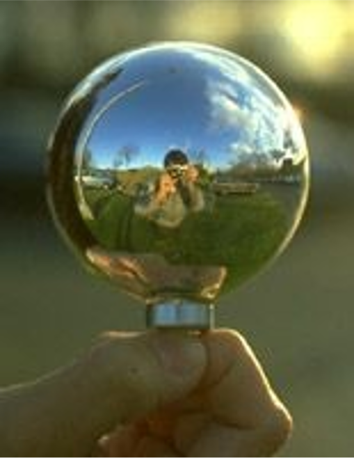
Environmental Mapping
Gazing balls
- Historical method from 1982 / 83
- I.e. photo of a reflecting sphere (gazing ball)
Methods to Create Environmental Maps
Environmental Mapping
360° Cameras / Panorama stitching apps
- Insta 360°, Facebook Surround 360°, etc.
- Microsoft Photosynth app, etc.
CGI Environmental Camera (e.g. OpenRT rt::CCameraEnvironment)
Methods to Create Environmental Maps

Procedural Textures
Procedural Textures
3D Textures
- Create a 3D parallelisation \((u,v,w) \) for the texture
- Map this onto the object
- The easiest parametrization is to use the model-space coordinate system to index into a 3D texture \((u,v,w) = (x, y, z)\)
- Like carving the object from the material
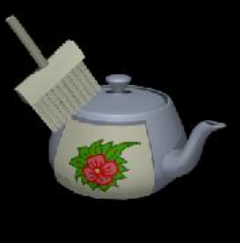
2D mapping
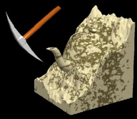
3D carving
3D Procedural Textures
Instead of using the texture coordinates as an index, use them to compute a function that defines the texture
\[f(u,v,w)\]
Procedural Textures
Example
Instead of an image, use a function
Vec3f CTextureProcedural::getVoxel(const Vec3f& uvw) const
{
    float u = uvw.val[0];	// hitpoint.x
    float v = uvw.val[1];	// hitpoint.y
    float w = uvw.val[2];	// hitpoint.z

    float k = 100;
    float intencity = (1 +  sinf(k * u) * cosf(k * v)) / 2;

    Vec3f color = Vec3f::all(intencity);

    return color;
}
Procedural Textures
Pros and Cons
Advantages over image texture
Disadvantages
- Infinite resolution and size
- More compact than texture maps
- No need to parameterise surface
- No worries about distortion and deformation
- Objects appear sculpted out of solid substance
- Can animate textures
- Difficult to match existing texture
- Not always predictable
- More difficult to code and debug
- Perhaps slower
- Aliasing can be a problem
Procedural Textures
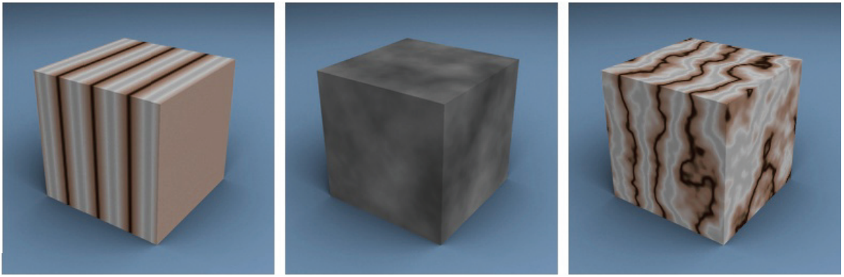
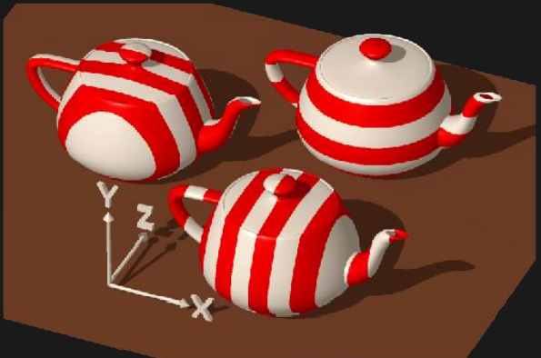
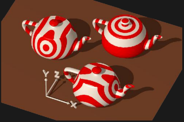
Simple Procedural Textures
Stripe
Rings
Color each point one or the other color depending on where \(floor(z)\) (or \(floor(x)\) or \(floor(y)\)) is even or odd
Color each point one or the other color depending on whether the \(floor(\) distancefrom object center along two coordinates\()\) is even or odd
Procedural Textures
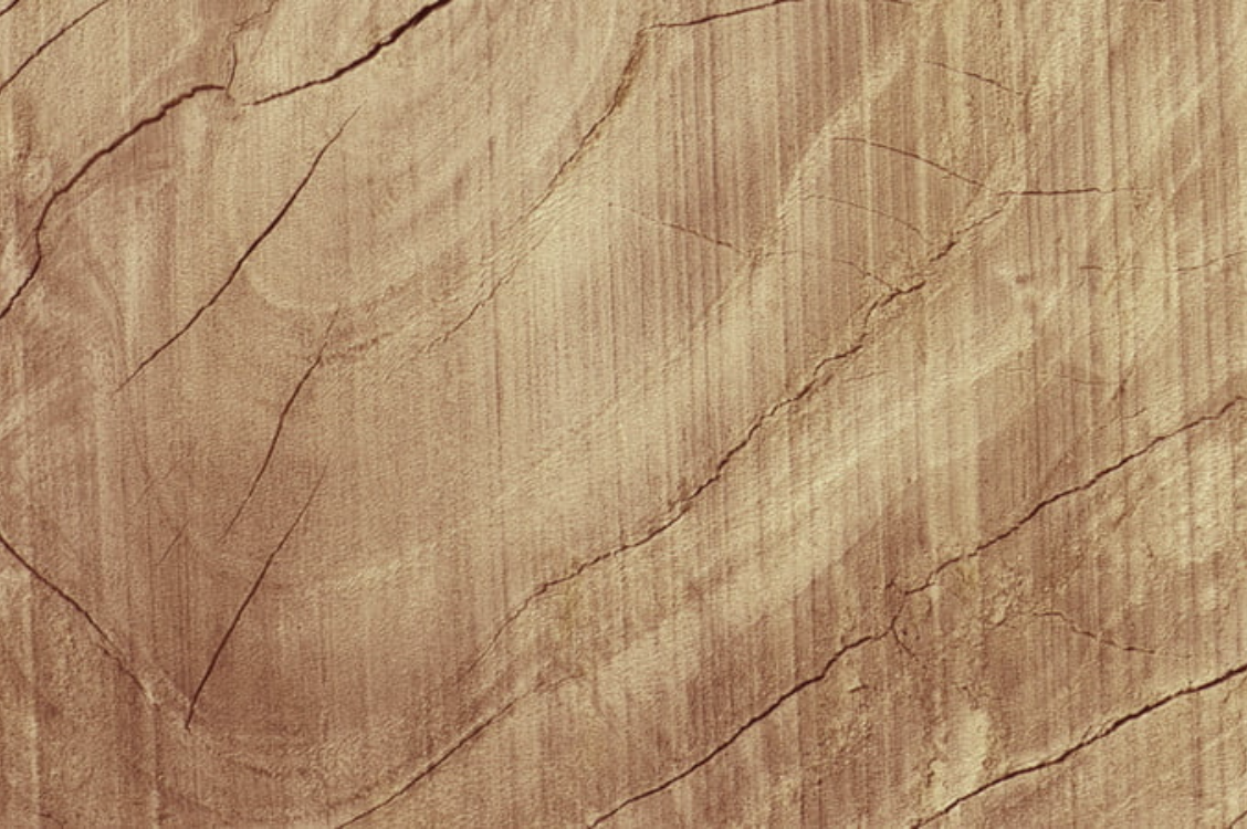
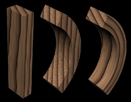
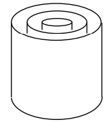
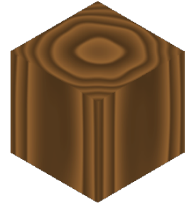
Wood Texture
Classify texture space into cylindrical shells
\[f(u,v,w) = (u^2+v^2)\]
Outer rings closer together, which simulates the growth rate of real trees.
Color look-up table
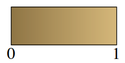
-
woodmap(0) -
woodmap(1)
= brown earlywood
= tan latewood
Wood texture
-
wood(u,v,w)=woodmap((u*u + v*v) % 1)
Procedural Textures
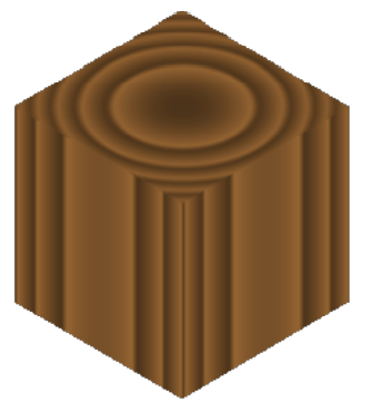
Wood Texture
Wood texture
-
wood(u,v,w)=woodmap((u*u + v*v) % 1)
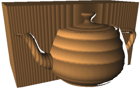
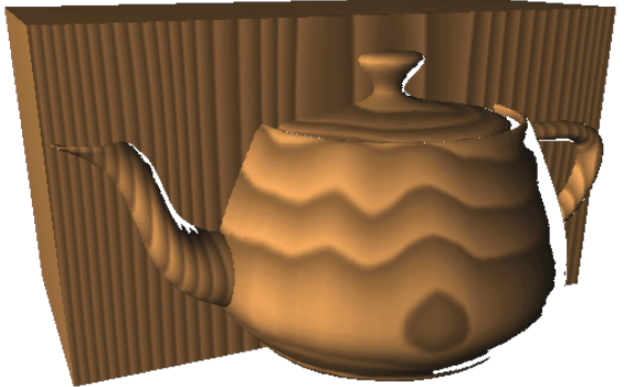
Adding noise
Add noise to cylinders to warp wood
-
wood(u,v,w)=woodmap((u*u + v*v) % 1 + noise(u,v,w))
\[noise(u,v,w)=\alpha\cdot noise(f_xu+\phi_x,f_yv+\phi_y,f_zw+\phi_z)\]
- Frequency (\(f\)): coarse vs. fine detail, number and thickness of noise peaks
- Phase (\(\phi\)): location of noise peaks
- Amplitude (\(\alpha\)): controls distortion due to noise effect
Procedural Textures
Wood Texture
Without noise
With noise
Procedural Textures
Perlin Noise
\(noise(u,v,w)\): pseudo-random number generator with the following characteristics:
- Memoryless
- Repeatable
- Isotropic
- Band limited (coherent): difference in values is a function of distance
- No obvious periodicity
- Translation and rotation invariant (but not scale invariant)
- Known range \([-1, 1]\)
- scale to \([0,1]\) using \(\frac{1 + noise()}{2}\)
- \(|noise()|\) creates dark veins at zero crossings
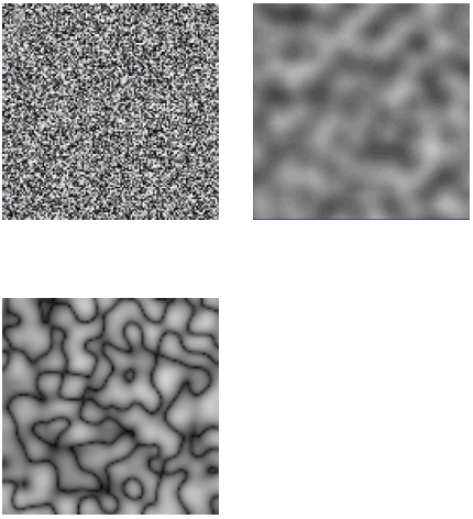
white noise
Perlin noise
Abs(Perlin noise)
Procedural Textures
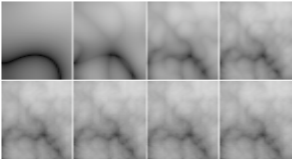
Turbulence
Fractal
Sum multiple calls to noise:
\[turbulance(u,v,w)=\sum^{octaves}_{i=1}\frac{1}{2^if}noise(2^if\cdot(u,v,w))\]
each additional term adds finer detail, with diminishing return
1-8 octaves of turbulence
Procedural Textures
Marble Texture
Use a sine function to create the stripes:
\[marble(u,v,w)=sin\left(f\cdot u+\alpha\cdot turbulance(u,v,w)\right)\]
- The frequency (\(f\)) of the sine function controls the number and thickness of the veins
- The amplitude (\(\alpha\)) of the turbulence controls the distortion of the veins