Multi-output spectral mixture Gaussian processes for lag estimation in multi-wavelength astronomical time series

Supervisors:

Dr Arash Bahramian, Dr Aloke Phatak,
Dr James Miller-Jones, Dr Suman Rakshit

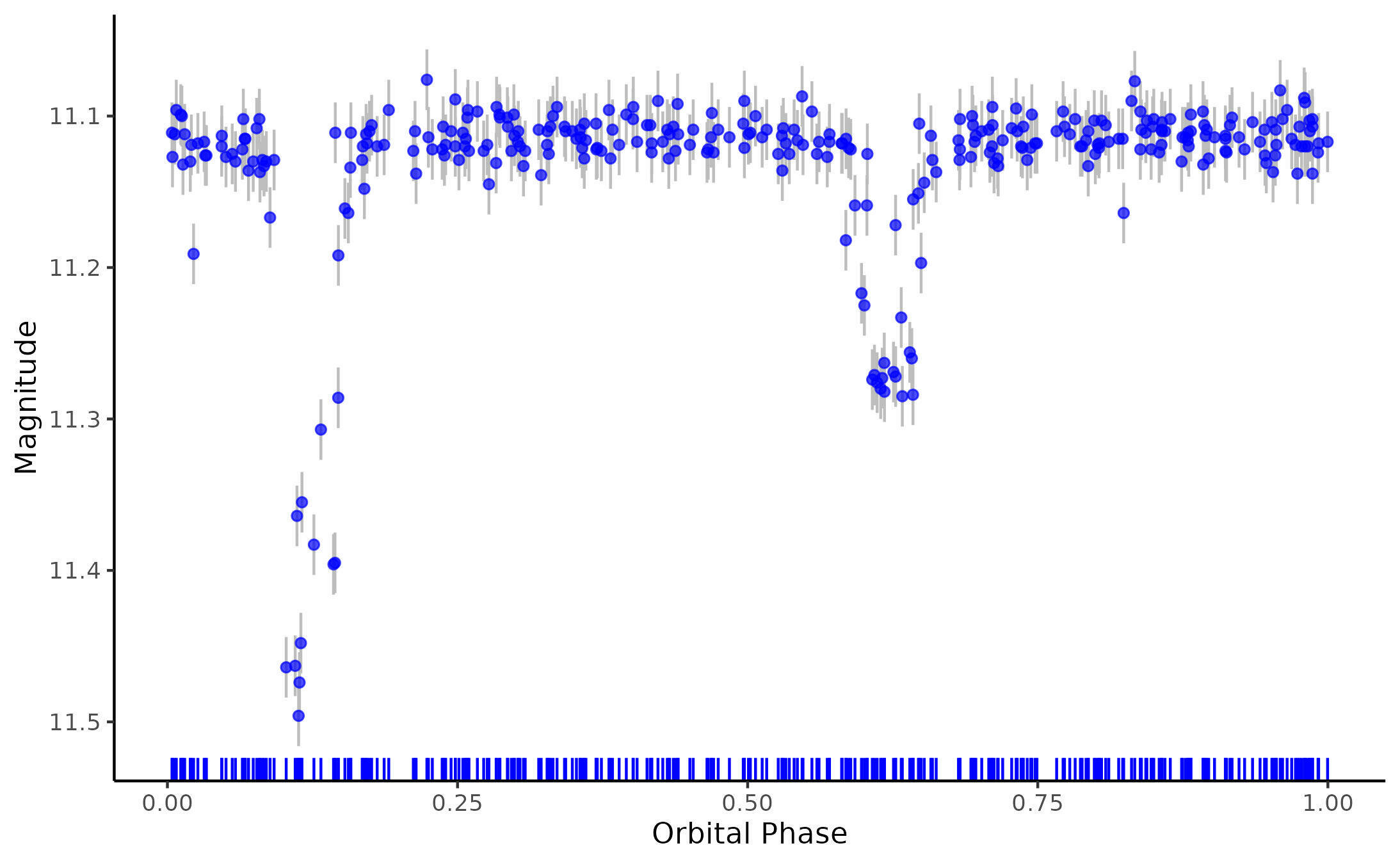
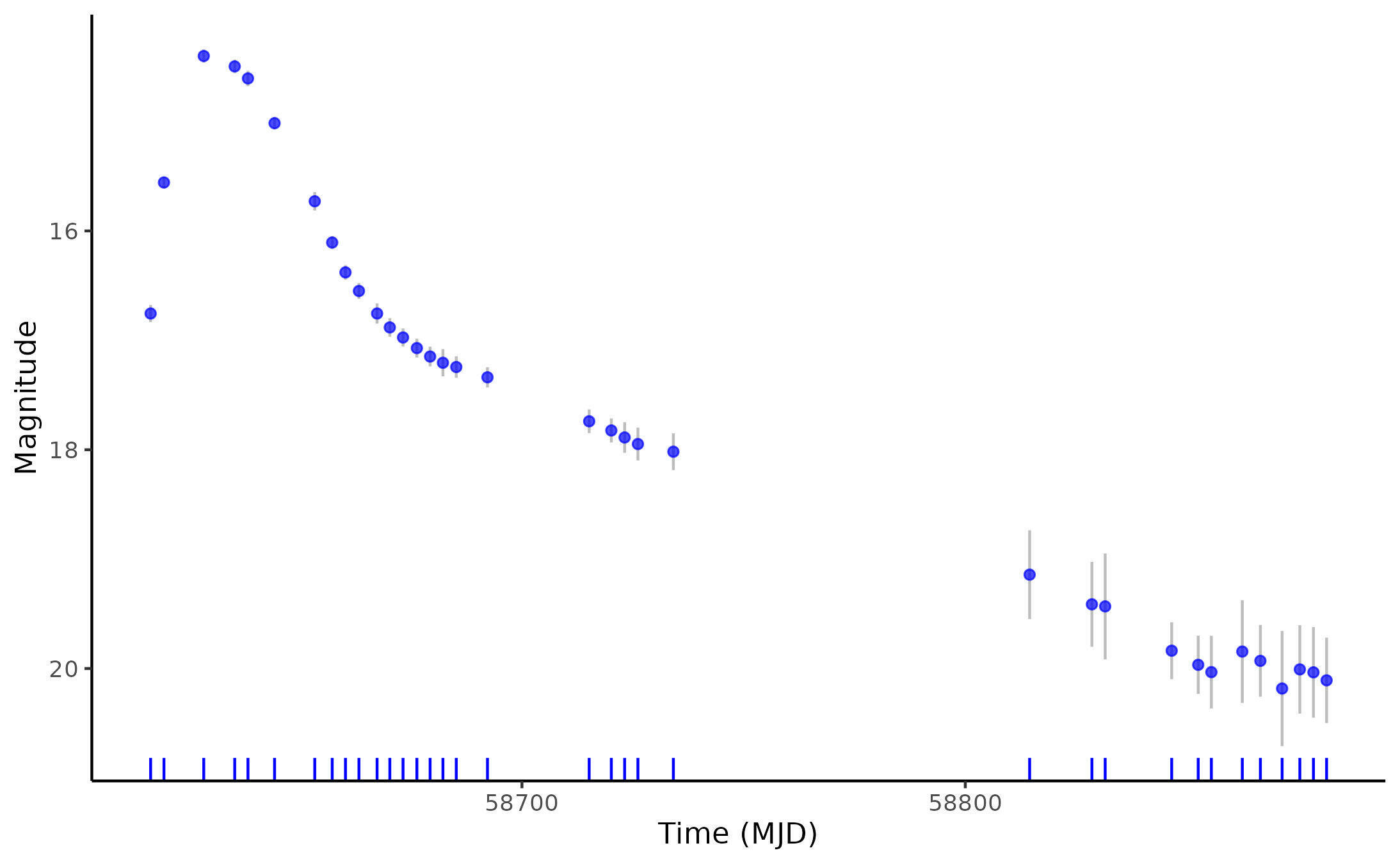
Light Curves

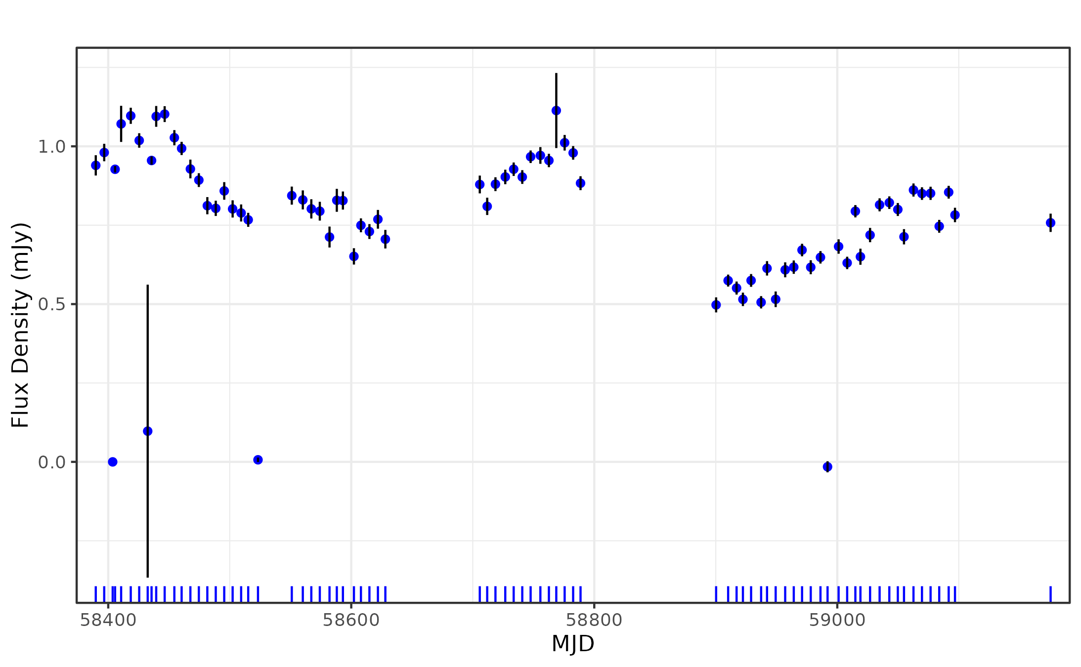
  • Light curves are time series data describing the changing brightest of a source over time.
  • The shape of a light curve can identify and reveal properties of the underlying object or event.
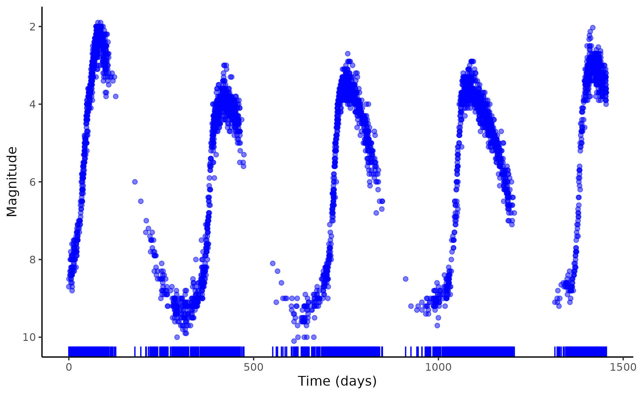
Treat the varying brightness of a source as a stochastic process

Magnitude

Magnitude

Magnitude

Time (days)

Orbital Phase

Time (MJD)

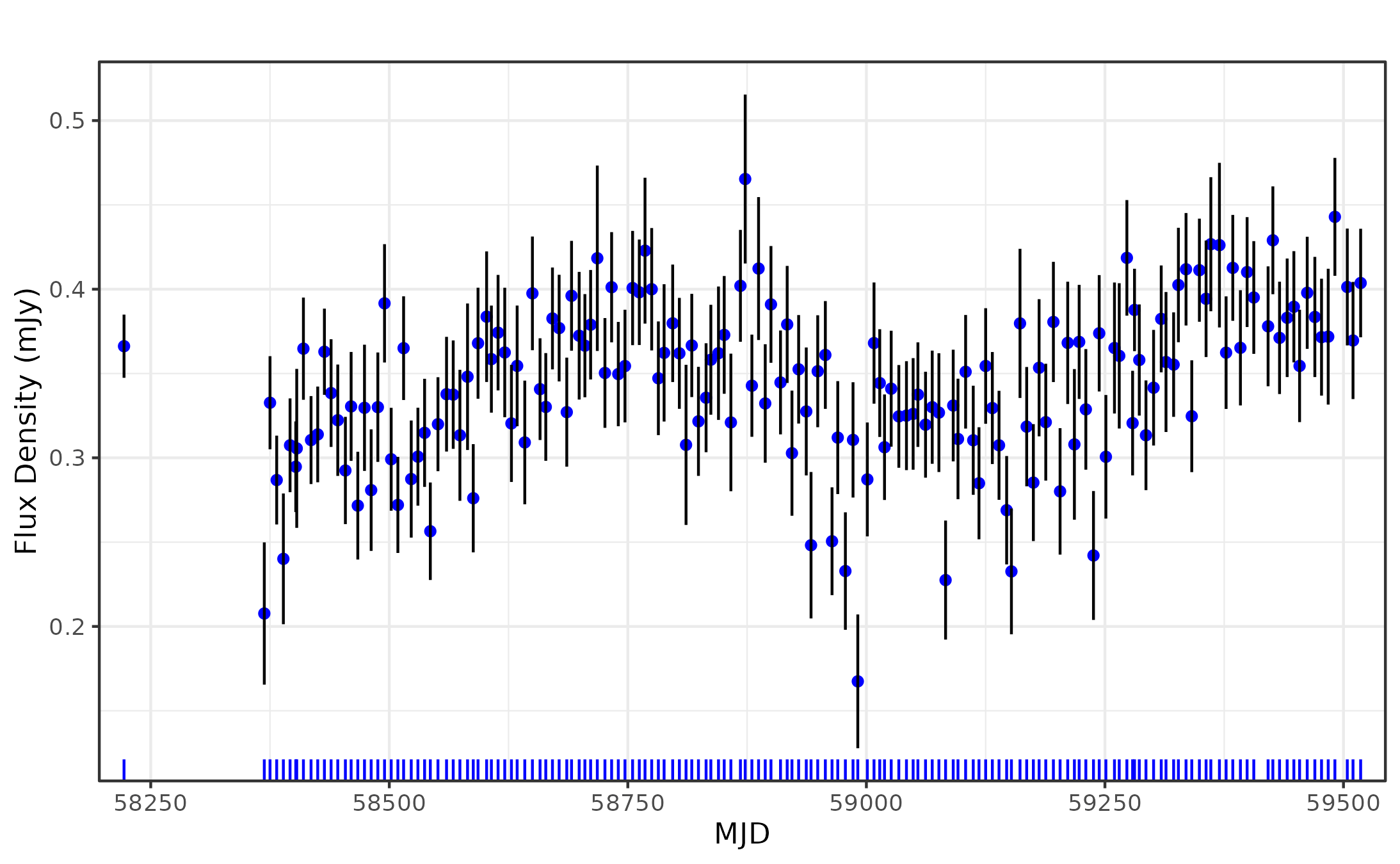
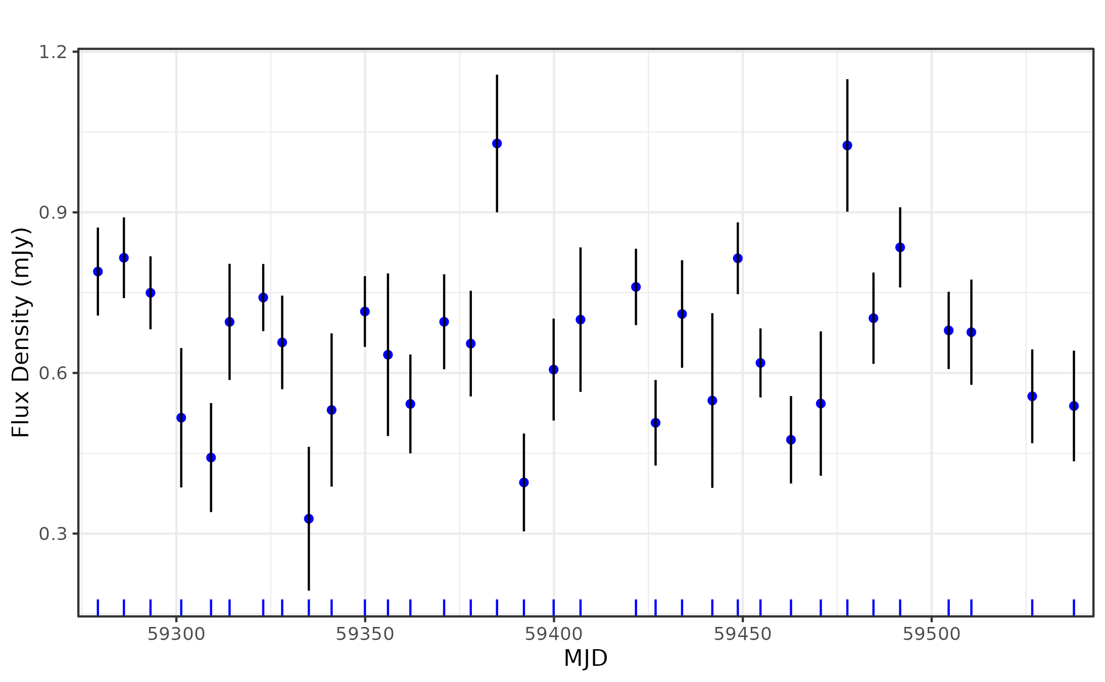
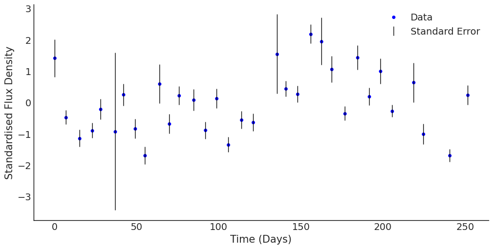
Heterogeneous Data

  • Different cadences
  • Sparse observations
  • Uneven sampling rates
  • Varying noise levels

Multivariate Normal

Y is a vector of n Gaussian distributed random variables.

\begin{bmatrix} Y_1 \\ \vdots \\ Y_n \end{bmatrix} \sim \mathcal{N}_n (\boldsymbol{\mu}, \boldsymbol{\Sigma}_{n \times n})
\boldsymbol{\Sigma}_{n \times n} = \begin{bmatrix} \Sigma_{11} & \dots & \Sigma_{1n} \\ \vdots & \ddots & \vdots \\ \Sigma_{n1} & \dots & \Sigma_{nn} \end{bmatrix}

where \(\boldsymbol\mu = (\mu_1, \dots, \mu_n)\) and \(\boldsymbol{\Sigma}\) is a \(n \times n \) covariance matrix.
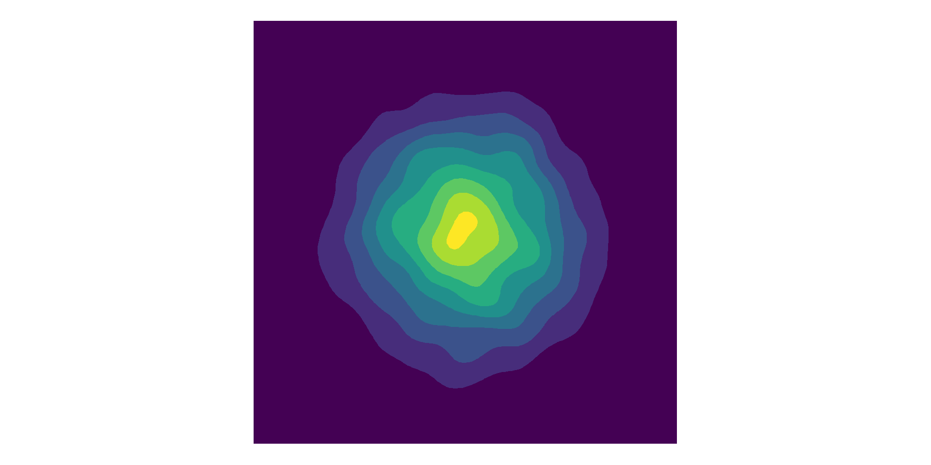
\mathbf{\Sigma} = \begin{bmatrix} 1 & 0 \\ 0 & 1 \end{bmatrix}
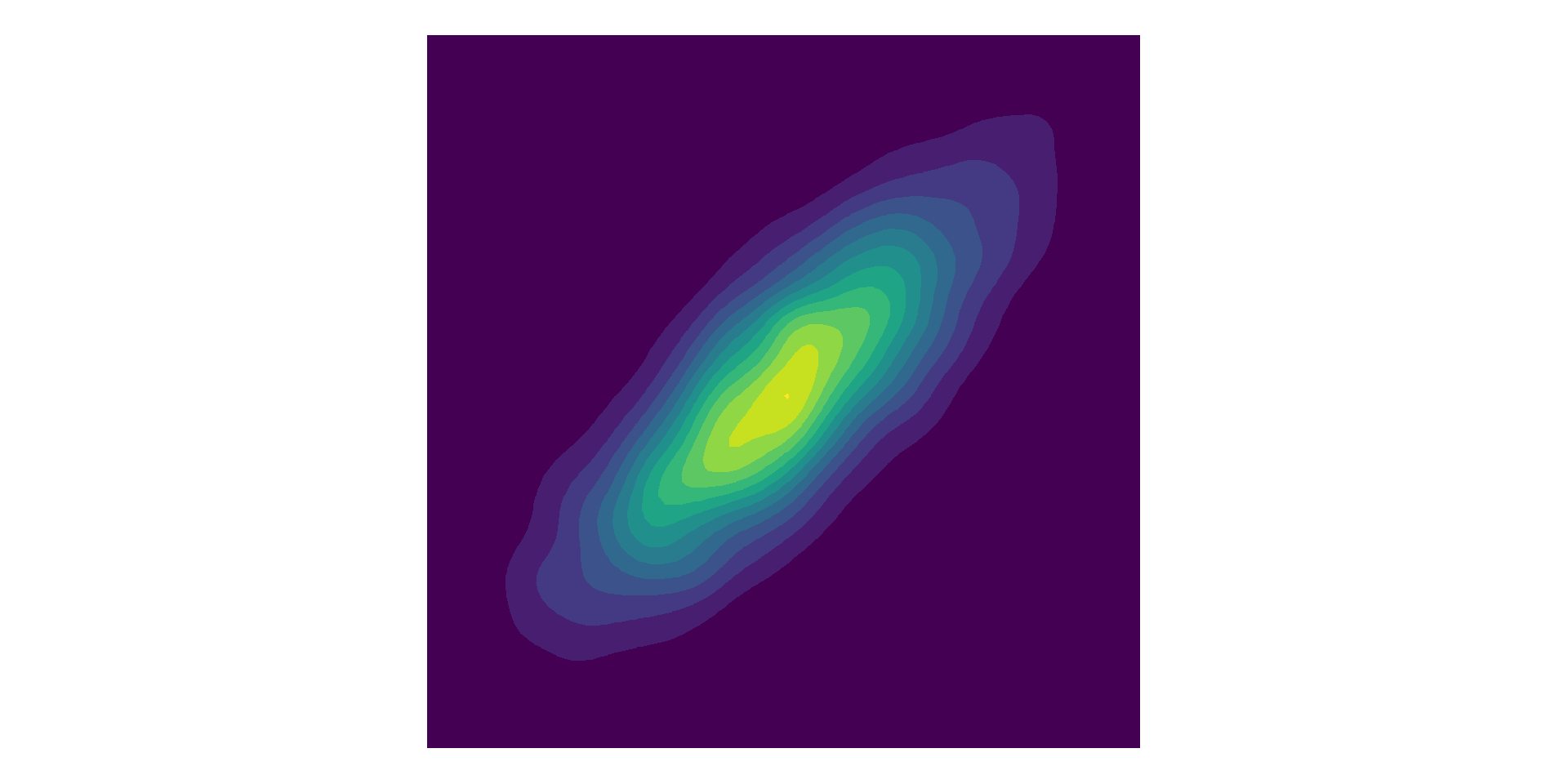
\mathbf{\Sigma} = \begin{bmatrix} 1 & 0.8 \\ 0.8 & 1 \end{bmatrix}
  • Symmetric, positive semi-definite matrix.
  • Linear combinations are also valid covariance matrices.

Gaussian Processes (GPs)

Extend multivariate Gaussian to 'infinite' dimensions.

  • Mean function, \(\mu(t)\)
  • Covariance or kernel function, \( \kappa(t,t'; \boldsymbol{\theta}) \)
\begin{bmatrix} Y_1 \\ Y_2 \\ \vdots \\ \end{bmatrix} \sim \mathcal{GP} (\mu(t), \boldsymbol{K})

where \(\mu = \mu(t)\) and \( K_{ij} = \kappa(t_i, t_j; \boldsymbol{\theta}) \), for \( i,j = 1, 2, \dots \)

Rather than specify a fixed covariance matrix with fixed dimensions, compute covariances using the kernel function.

\boldsymbol{K} = \begin{bmatrix} K_{11} & \dots & K_{1.} \\ \vdots & \ddots & \vdots \\ K_{.1} & \dots & K_{..} \end{bmatrix}

Gaussian Process Regression

f(\boldsymbol{x}) \sim \mathcal{GP}(\boldsymbol{0}, \kappa(\boldsymbol{x}, \boldsymbol{x}'; \boldsymbol{\theta}))
y(\boldsymbol{x}_i) = f(\boldsymbol{x}_i) + \varepsilon_i
\varepsilon_i \sim \mathcal{N}(0, \sigma^2)
\begin{bmatrix} y(\boldsymbol{x}_1)\\ \vdots \\ y(\boldsymbol{x}_n) \end{bmatrix} \sim \mathcal{N}\left(\begin{bmatrix}0\\ \vdots \\ 0 \end{bmatrix}, \begin{bmatrix} \kappa(\boldsymbol{x}_1, \boldsymbol{x}_1) & \dots & \kappa(\boldsymbol{x}_1, \boldsymbol{x}_n) \\ \vdots & \ddots & \vdots \\ \kappa(\boldsymbol{x}_n, \boldsymbol{x}_1) & \dots & \kappa(\boldsymbol{x}_n, \boldsymbol{x}_n) \end{bmatrix} + \sigma^2 \begin{bmatrix} 1 & \dots & 0 \\ \vdots & \ddots & \vdots \\ 0 & \dots & 1 \end{bmatrix}\right)
\boldsymbol{y} \sim \mathcal{N}(\boldsymbol{0}, \boldsymbol{K} + \sigma^2 \boldsymbol{I})

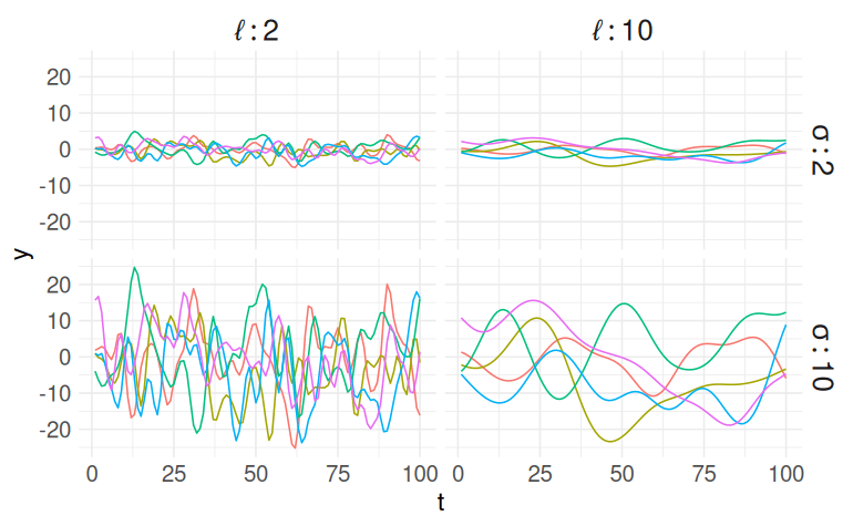
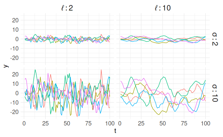
Kernel Functions

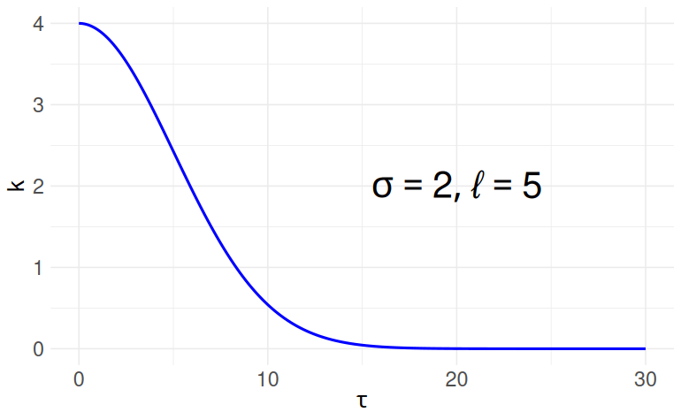
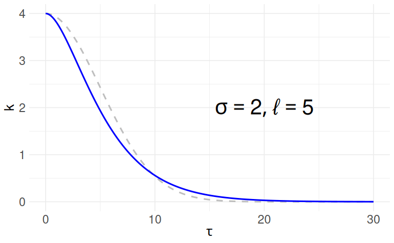
Squared Exponential

Matern 3/2

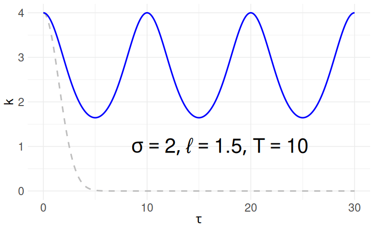
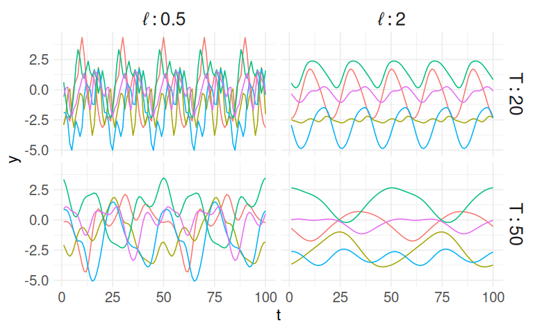
Periodic

\tau = | t_r - t_c |; \sigma, \ell, T > 0

$$\kappa(\tau; \sigma, \ell) = \sigma^2 \exp\left\{ -\frac{1}{2}\left( \frac{\tau}{\ell}\right)^2\right\}$$

$$\kappa(\tau; \sigma, \ell) = \sigma^2 \left( 1 + \sqrt{3}\frac{\tau}{\ell}\right) \exp\left\{ - \sqrt{3} \frac{\tau}{\ell}\right\}$$

$$\kappa(\tau; \sigma, \ell, T) = \sigma^2 \exp\left\{ -\frac{2}{\ell^2} \sin^2\left( \pi \frac{\tau}{T}\right)\right\}$$

Squared Exponential (Gaussian) Kernel
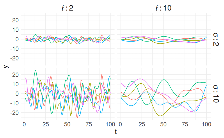
\kappa(\tau; \sigma, \ell) = \sigma^2 \exp\left\{ -\frac{1}{2}\left( \frac{\tau}{\ell}\right)^2\right\}
\tau = | t_r - t_c | \\ \sigma, \ell > 0

Bayesian Hierarchical Model

\begin{gather*} i, r,c = 1, \dots, n.\\ \boldsymbol\theta = (\sigma_\mathrm{SE}, \ell_\mathrm{SE}, \sigma_\mathrm{M32}, \ell_\mathrm{M32}, \sigma_\mathrm{P}, \ell_\mathrm{P}, T) \end{gather*}
\begin{align*} [\boldsymbol\Sigma]_{r,c} &= \kappa(t_r - t_c \mid \boldsymbol{\theta})\\ &= \kappa_1(\tau; \sigma_\mathrm{SE}, \ell_\mathrm{SE}) + \kappa_2(\tau; \sigma_\mathrm{M32}, \ell_\mathrm{M32}) + \kappa_3(\tau; \sigma_\mathrm{P}, \ell_\mathrm{P}, T) \end{align*}

Squared Exponential

Matern 3/2

Periodic

\(Y_i \sim \mathcal{N}\left(f_i, \hat{e_i}^2\right)\)

\(\boldsymbol{f} \sim \mathcal{GP}\left(\boldsymbol{0}, \boldsymbol{\Sigma}_{n \times n}\right)\)

Hyperparameters

Respone

GP prior

"Single-output" GP
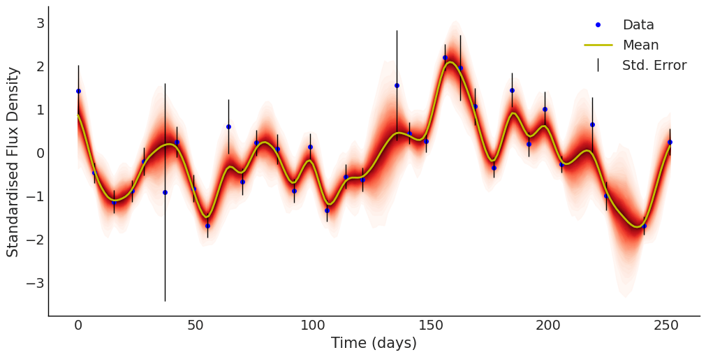
\sigma_\mathrm{SE} = 0.37\\ \ell_\mathrm{SE} = 48.1\\ \sigma_\mathrm{M32} = 1.21\\ \ell_\mathrm{M32} = 12.4\\ \sigma_\mathrm{P} = 0.45\\ \ell_\mathrm{P} = 47.1\\ T = 26.1

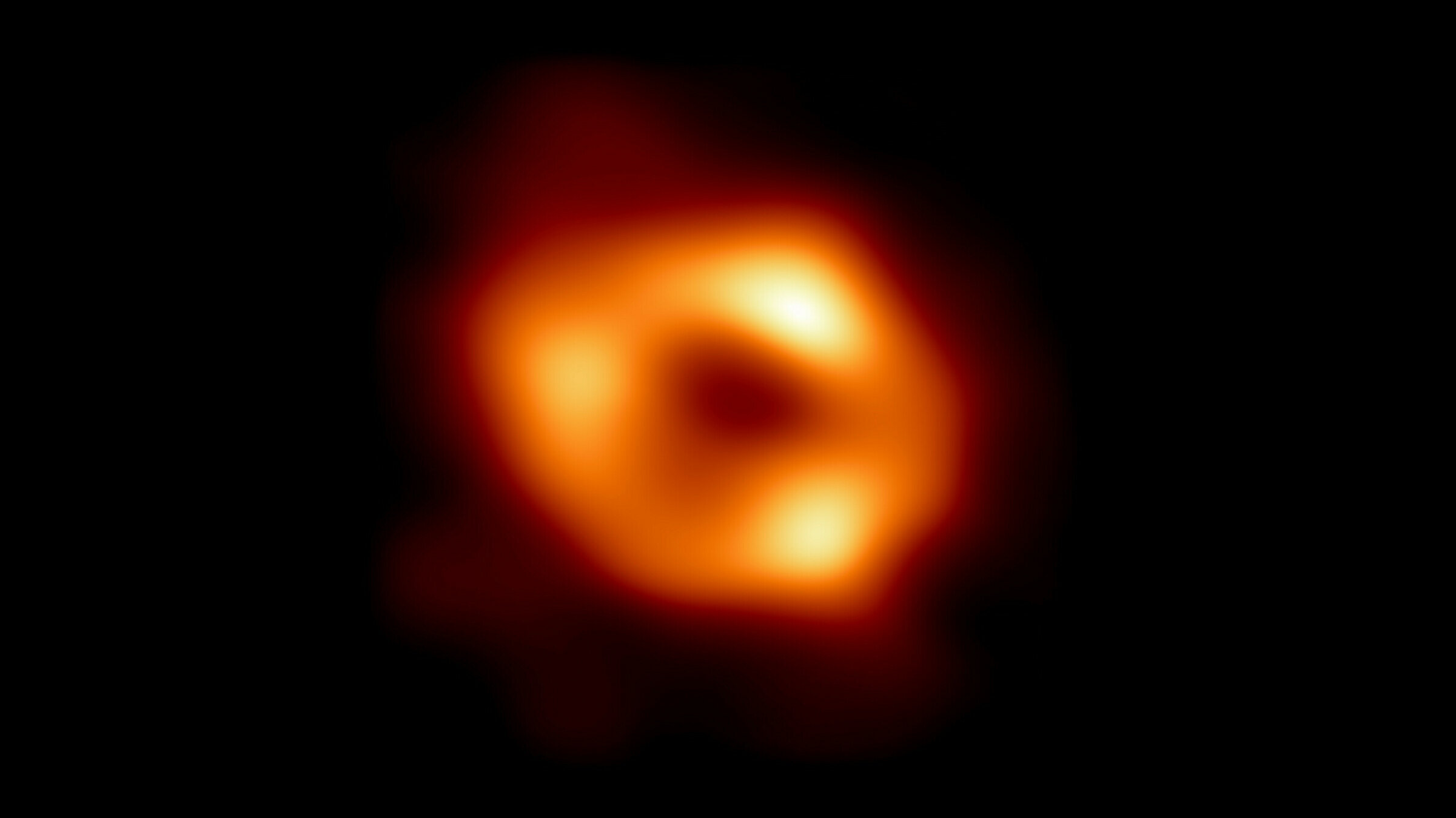
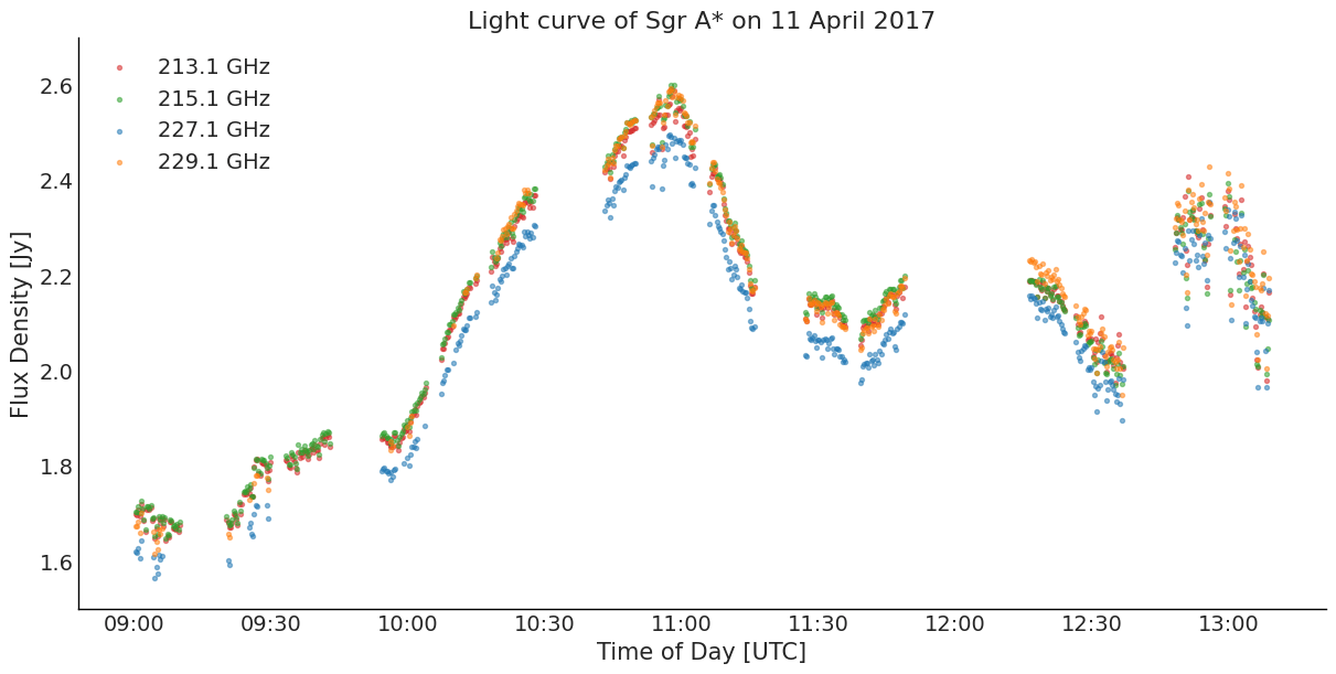
Sagittarius A* (Sgr A*)

  • Supermassive Black Hole (SMBH) at the centre of the Milky Way.
  • 4 million solar masses.
  • ~27,000 ly from Earth
  • Image created from observations taken in 2017 by the Event Horizon Telesope (EHT) Collaboration.

Image credit: EHT Collaboration

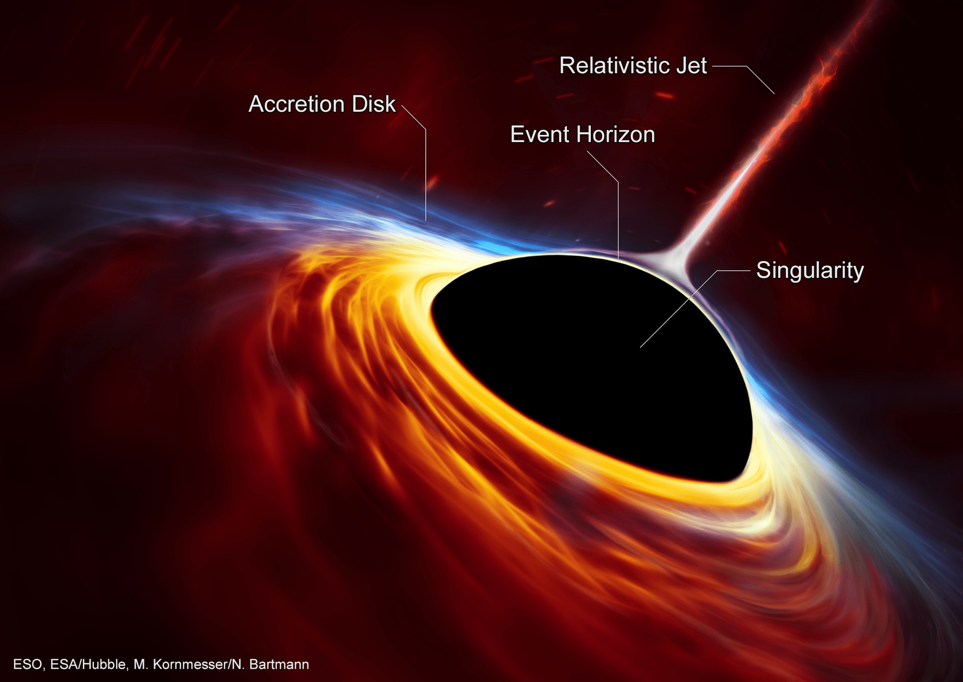
Anatomy of a Black Hole

Multi-band time-domain astronomy

  1. Estimate the characteristic timescales of the variability in the black hole emissions.
  2. Characterise the relationship between emissions of different wavelengths, e.g, time delay between bands.
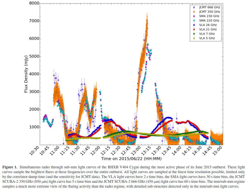
Credit: Tetarenko et al. (2017)

Black hole X-ray binary

V404 Cygni

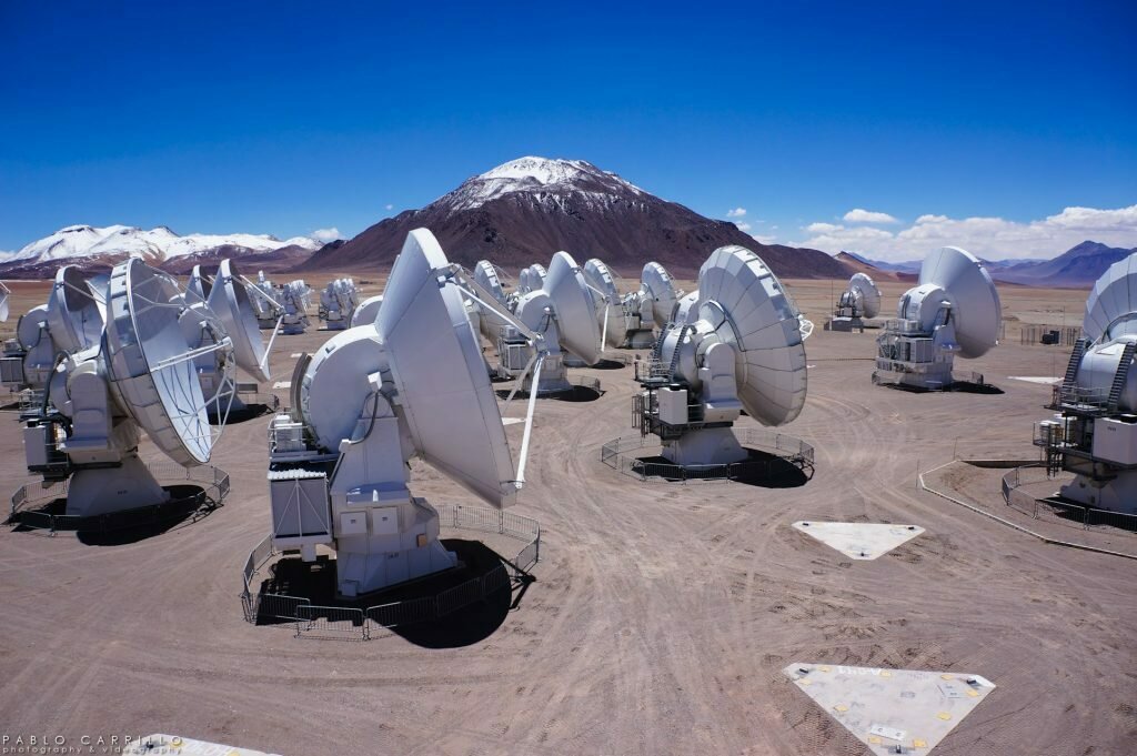
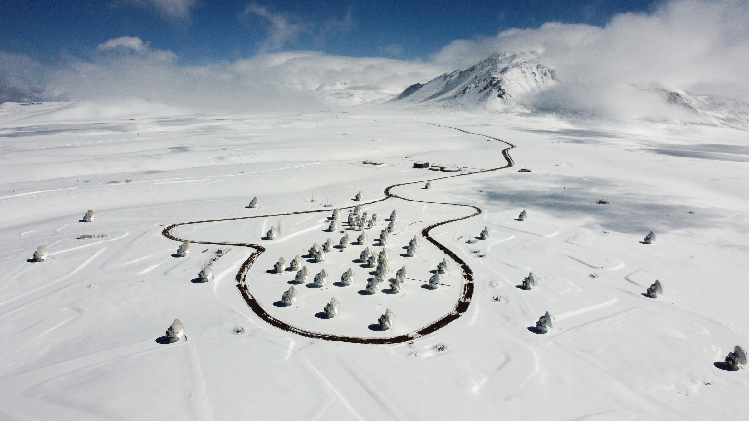
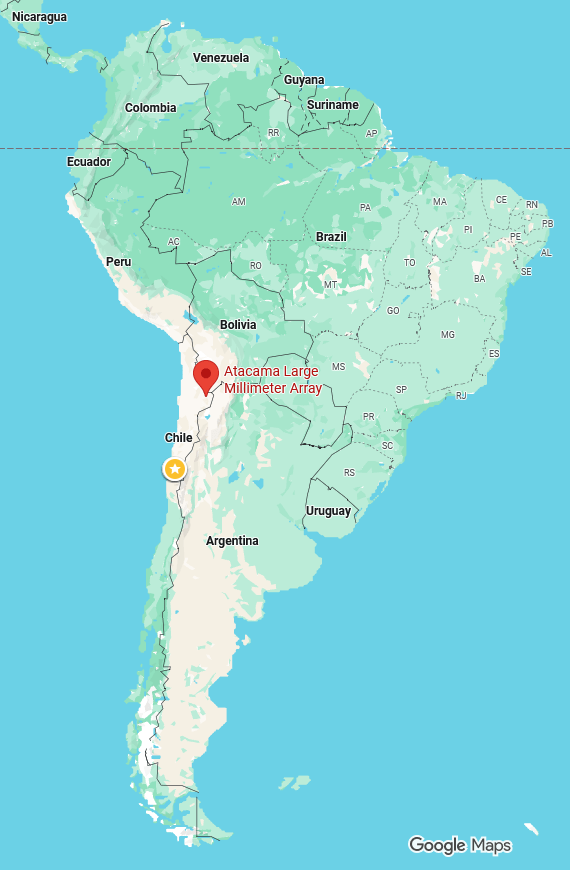
Atacama Large Millimeter Array (ALMA)

  • Chilean Atacama Desert at 5000m elevation.
  • 66 high-precision dish antennas: 54 x 12m and 12 x 7m across.
  • Radio and infrared.
  • Member site of EHT Collaboration.

Credit: NRAO/AUI/NSF

Multi-band Light Curve

Multi-Output GP (MOGP)

\begin{bmatrix} \boldsymbol{y}_1\\ \boldsymbol{y}_2 \end{bmatrix} \sim \mathcal{N}\left(\begin{bmatrix}\boldsymbol{0}\\ \boldsymbol{0} \end{bmatrix}, \begin{bmatrix} \boldsymbol{K}_1 & \boldsymbol{0} \\ \boldsymbol{0} & \boldsymbol{K}_2 \end{bmatrix} + \begin{bmatrix} \sigma^2_1 \boldsymbol{I} & \boldsymbol{0} \\ \boldsymbol{0} & \sigma^2_2 \boldsymbol{I} \end{bmatrix}\right)
\boldsymbol{y} \sim \mathcal{N}(\boldsymbol{0}, \boldsymbol{K}_{\boldsymbol{f},\boldsymbol{f}} + \boldsymbol{\Sigma})

\((n_1 + n_2) \times 1\)

\((n_1 + n_2) \times (n_1 + n_2)\)

Cross-covariance

\(\boldsymbol{K}_{\boldsymbol{f},\boldsymbol{f}}\)

f_1(\boldsymbol{x}) \sim \mathcal{GP}(\boldsymbol{0}, \kappa_1(\boldsymbol{x}, \boldsymbol{x}'))
\boldsymbol{y}_1 \sim \mathcal{N}(\boldsymbol{0}, \boldsymbol{K}_1 + \sigma^2_1 \boldsymbol{I})
\mathcal{D}_1 = \{ ( \boldsymbol{x}_{i,1}, y_1(\boldsymbol{x}_{i,1}) ) ; i = 1, \dots, n_1\}
f_2(\boldsymbol{x}) \sim \mathcal{GP}(\boldsymbol{0}, \kappa_2(\boldsymbol{x}, \boldsymbol{x}'))
\boldsymbol{y}_2 \sim \mathcal{N}(\boldsymbol{0}, \boldsymbol{K}_2 + \sigma^2_2 \boldsymbol{I})
\mathcal{D}_2 = \{ ( \boldsymbol{x}_{i,2}, y_2(\boldsymbol{x}_{i,2}) ) ; i = 1, \dots, n_2\}

MOGP Kernels

  • Choose a cross-covariance function \( \operatorname{cov}[f_1(\boldsymbol{x}),f_2(\boldsymbol{x}')]\) such that \( \boldsymbol{K}_{\boldsymbol{f},\boldsymbol{f}}\) is a valid covariance matrix, i.e., positive semi-definite.
  • Many forms of "separable" kernels where \(\boldsymbol{K}_{\boldsymbol{f},\boldsymbol{f}}\) is decomposed into submatrices, e.g., LMC, ICM, SLFM, see Alvarez et al. (2012).
\begin{bmatrix} \boldsymbol{f}_1\\ \boldsymbol{f}_2 \end{bmatrix} \sim \mathcal{N}\left(\begin{bmatrix}\boldsymbol{0}\\ \boldsymbol{0} \end{bmatrix}, \begin{bmatrix} \boldsymbol{K}_1 & \\ & \boldsymbol{K}_2 \end{bmatrix} + \begin{bmatrix} \sigma^2_1 \boldsymbol{I} & \boldsymbol{0} \\ \boldsymbol{0} & \sigma^2_2 \boldsymbol{I} \end{bmatrix}\right)

\(\boldsymbol{K}_{\boldsymbol{f},\boldsymbol{f}}\)

?

?

Semiparametric Latent Factor Model (SLFM)

Fit each band as a linear combination of two latent GPs,

where \(d = 1,2\) output bands and \(q = 1,2\) latent processes

\begin{align*} \begin{bmatrix} \boldsymbol{f}_1\\ \boldsymbol{f}_2 \end{bmatrix} &= \begin{bmatrix} a_{1,1} & a_{1,2} \\ a_{2,1} & a_{2,2} \end{bmatrix} \times \begin{bmatrix} u_1(\boldsymbol{x}) \\ u_2(\boldsymbol{x}) \end{bmatrix} = \begin{bmatrix} \boldsymbol{a}_1 & \boldsymbol{a}_2 \end{bmatrix} \times \begin{bmatrix} u_1(\boldsymbol{x}) \\ u_2(\boldsymbol{x}) \end{bmatrix} \end{align*}
\boldsymbol{f}(\boldsymbol{x}) = \boldsymbol{a}_1 u_1 (\boldsymbol{x}) + \boldsymbol{a}_1 u_2 (\boldsymbol{x})
\begin{align*} u_1(\boldsymbol{x}) &\sim \mathcal{GP}(\boldsymbol{0}, \kappa_1(x, x'))\\ u_2(\boldsymbol{x}) &\sim \mathcal{GP}(\boldsymbol{0}, \kappa_2(x, x')) \end{align*}
f_d(\boldsymbol{x}) = \sum^2_q a_{d,q} u_q(\boldsymbol{x})

Alternatively,

Semi-parametric Latent Factor kernel

\begin{align*} \boldsymbol{K}_{\boldsymbol{f},\boldsymbol{f}} &= \begin{bmatrix} \mathrm{cov}[f_1(\boldsymbol{x}), f_1(\boldsymbol{x'})] & \dots & \mathrm{cov}[f_1(\boldsymbol{x}), f_4(\boldsymbol{x'})]\\ \vdots & \ddots & \vdots \\ \mathrm{cov}[f_1(\boldsymbol{x'}), f_4(\boldsymbol{x})] & \dots & \mathrm{cov}[f_4(\boldsymbol{x}), f_4(\boldsymbol{x'})] \end{bmatrix} \\ &= \sum^2_q \boldsymbol{a}_q \boldsymbol{a}_q^\top \otimes \kappa_q(\boldsymbol{x}, \boldsymbol{x}') \\ &= \sum^2_q \boldsymbol{B}_q \otimes \boldsymbol{K}_{f_q, f_q} \end{align*}

Co-regionalisation Matrices

Kronecker product

  • Cross-covariance between channels is the same shape as the auto-covariance.

  • Cannot model any lag between channels.

Spectral Mixture Kernel

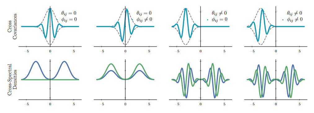
  • Design a multi-output kernel in the spectral (Fourier) domain rather than in the time domain.
  • Cramer's Theorem guarantees a valid kernel in the time-domain if the matrix of cross-spectral densities \(\mathbf{S}(\omega) \) is
    • Hermitian,
    • positive semi-definite, and
    • integrable
  • Alternatively:
    • non-negative
    • symmetrical about origin

(Figure adapted from Parra & Tobar 2017)

Spectral Mixture Kernel

Closed-form covariance functions after inverse Fourier transform.

k_{ij}(\tau) = \sum_{q=1}^{Q} \alpha_{ij}^{(q)} \exp\!\Big(-\tfrac{1}{2}\,\Sigma_{ij}^{(q)}\big(\tau + \theta_{ij}^{(q)}\big)^2\Big) \cos\!\Big(\mu_{ij}^{(q)}\big(\tau + \theta_{ij}^{(q)}\big) + \phi_{ij}^{(q)}\Big)

For \(Q\) spectral components, the covariance between bands \(i\) and \(j\) at lag \(\tau = t - t'\) is

k_{ij}(\tau) = \alpha_{ij} \exp\!\Big(-\tfrac{1}{2}\,\Sigma_{ij}\big(\tau + \theta_{ij}\big)^2\Big) \cos\!\Big(\mu_{ij}\big(\tau + \theta_{ij}\big) + \phi_{ij}\Big)

For a single component, \(Q = 1\):

"Squared Exponential envelope"

Periodic oscillation

Spectral Mixture Kernel

k_{ij}(\tau) = \alpha_{ij} \exp\!\Big(-\tfrac{1}{2}\,\Sigma_{ij}\big(\tau + \theta_{ij}\big)^2\Big) \cos\!\Big(\mu_{ij}\big(\tau + \theta_{ij}\big) + \phi_{ij}\Big)

The cross-band parameters are built from the per-band weight \(w_i\), spectral mean \(\mu_i\), spectral variance \(\Sigma_i\), delay \(\theta_i\) and phase \(\phi_i\):

\Sigma_{ij} = \frac{2\,\Sigma_i\Sigma_j}{\Sigma_i + \Sigma_j} \\

Width of cross-covariance envelope

\theta_{ij} = \theta_i - \theta_j

Delay between bands

\phi_{ij} = \phi_i - \phi_j

Phase offset

\mu_{ij} = \frac{\Sigma_j\mu_i + \Sigma_i\mu_j}{\Sigma_i + \Sigma_j}

Oscillation frequency of cross-covariance

w_{ij} = w_i w_j \exp\!\left\{-\frac{\big(\mu_i - \mu_j\big)^2}{4\big(\Sigma_i + \Sigma_j\big)}\right\}

Strength of coupling between bands

\alpha_{ij} = w_{ij}\sqrt{2\pi\,\Sigma_{ij}}

Amplitude of cross-covariance

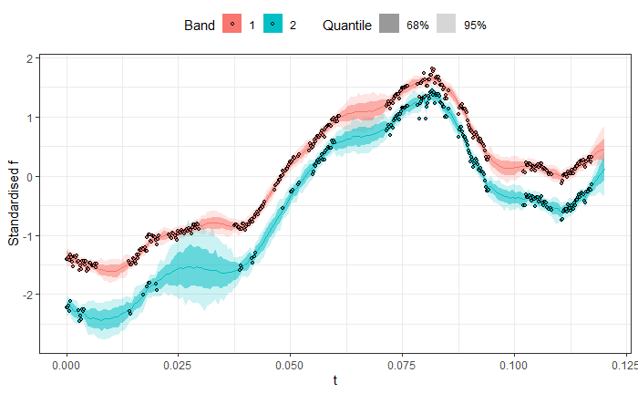
Four-band Light Curve

Two-band Light Curve
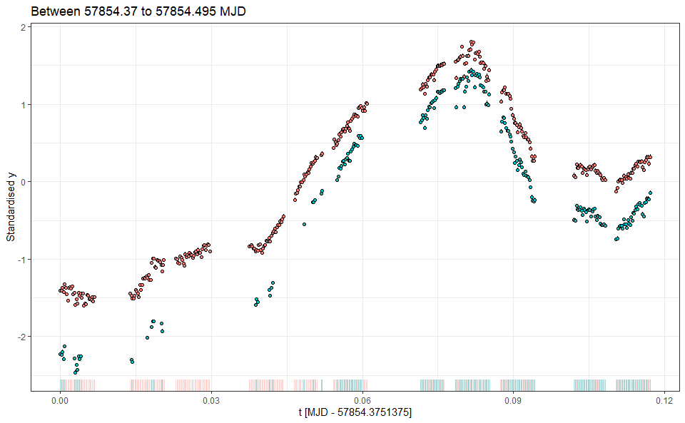
Two-output MOGP Model

\mathbf{y} = \begin{pmatrix} \mathbf{y}_1 \\ \mathbf{y}_2 \end{pmatrix} \in \mathbb{R}^{M}, \qquad \mathbf{y}_i = (y_{i,1},\dots,y_{i,N_i})^\top, \qquad M = N_1 + N_2
y_{i,n} = f_i(t_{i,n}) + \varepsilon_{i,n}, \qquad \varepsilon_{i,n} \sim \mathcal{N}(0, \sigma_{i,n}^2),
\mathbf{f} = (f_1, f_2)
\operatorname{cov}\big(f_i(t), f_j(t')\big) = k_{ij}(t - t')
\mathbf{y} \mid \boldsymbol{\Theta} \sim \mathcal{N}\!\big(\mathbf{0},\; \mathbf{K} + \mathbf{D}), \qquad \mathbf{D} = \operatorname{diag}\big(\sigma_{1,1}^2,\dots,\sigma_{1,N_1}^2, \sigma_{2,1}^2,\dots,\sigma_{2,N_2}^2\big)
\mathbf{K} = \begin{pmatrix} \mathbf{K}_{11} & \mathbf{K}_{12} \\ \mathbf{K}_{12}^\top & \mathbf{K}_{22} \end{pmatrix}, \qquad [\mathbf{K}_{ij}]_{n,m} = k_{ij}\big(t_{i,n} - t_{j,m}\big)

Data Model

Process Model

\boldsymbol{\Theta} = \Big\{\Sigma_i,\ \mu_i, w_i, \theta_i, \phi_i\Big\}_{i \in \{1,2\}}

Parameter Model

\Sigma_i = \big(\ell_i\big)^{-2}, \qquad \ell_{\min} \le \ell_i \le \ell_{\max}
v_i^{(q)} = k_{ii}^{(q)}(0) = \big(w_i^{(q)}\big)^2\sqrt{2\pi\,\Sigma_i^{(q)}}
v_i^{(q)} = \varsigma_i^{2}\, s_i^{(q)}, \qquad \mathbf{s}_i = \big(s_i^{(1)},\dots,s_i^{(Q)}\big) \in \Delta^{Q-1}, \sum_{q=1}^{Q} s_i^{(q)} = 1

length-scale in time

variance contribution of component \(q\)

split from total variance of band \(i\)

\theta_1^{(q)} = \phi_1^{(q)} = 0, \qquad \theta_2^{(q)} \equiv \vartheta_q \in \mathbb{R}, \qquad \phi_2^{(q)} \equiv \varphi_q \in (-\pi, \pi),

Identifiability constraints

0 < \mu_1^{(1)} < \mu_1^{(2)} < \dots < \mu_1^{(Q)}, \qquad \mu_2^{(q)} > 0 \ \ (q = 1,\dots,Q).

Priors

\begin{align*} \varsigma_i &\sim \mathrm{lognormal}\big(0,\ \tau_\varsigma^2\big), && i = 1,2, \\ \mathbf{s}_i &\sim \mathrm{Dirichlet}\big(a\,\mathbf{1}_Q\big), && i = 1,2, \\ \big(\mu_1^{(1)},\dots,\mu_1^{(Q)}\big) &\sim \prod_{q=1}^{Q}\N\big(\mu_1^{(q)} \mid 0, \tau_\mu^2\big)\, \mathbf{I}\big[0 < \mu_1^{(1)} < \dots < \mu_1^{(Q)}\big], \\ \mu_2^{(q)} &\sim \mathcal{N}^{+}\big(0,\ \tau_\mu^2\big), && q = 1,\dots,Q, \\ \ell_i^{(q)} &\sim \mathrm{lognormal}\big(m_\ell,\ s_\ell^2\big)\ \text{truncated to } [\ell_{\min}, \ell_{\max}], && i = 1,2,\ q = 1,\dots,Q, \\ \vartheta_q &\sim \mathcal{N}(0, 1), && q = 1,\dots,Q, \\ \varphi_q &\sim \mathrm{Unif}(-\pi, \pi), && q = 1,\dots,Q, \end{align*}

Posterior Predictive Curves

Hyperparameter Posteriors
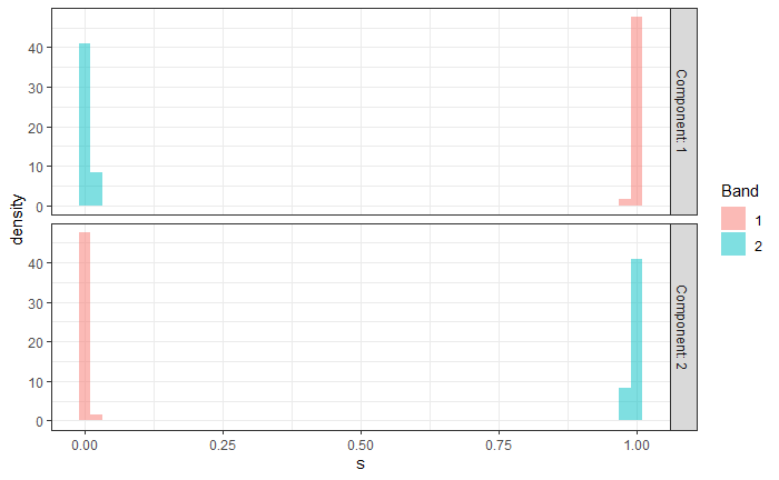
\(s_{q,i}\) is the share of a band \(i\)’s signal variance carried by component \(q\).

  • Band 1 is almost completely encoded by Component 1
  • Band 2 is almost completely encoded by Component 2

Hyperparameter Posteriors

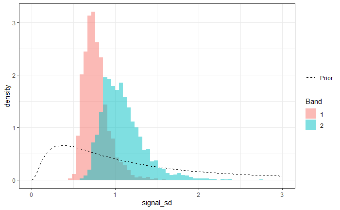
\(\varsigma_i\) is the total standard deviation of the signal captured in band \(i\) .

  • There is a reasonable sharing of signal variance between both bands.
Hyperparameter Posteriors

\(\ell_{q,i}\) is the length scale of Component \(q\) band \(i\) .

  • Component 1 has a length scale of approximately 11 minutes.
  • Component 2 has a length scale of approximately 14 minutes.
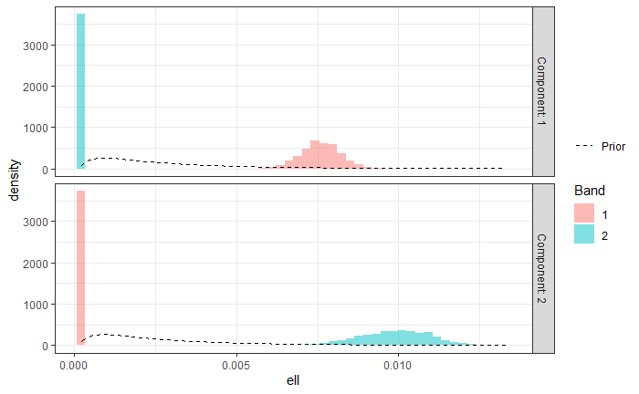
Band 1Band 2
Component 10.00760.0002
Component 20.00020.010

Hyperparameter Posteriors

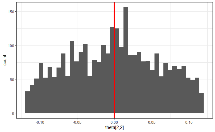
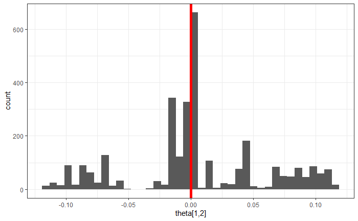
\(\vartheta_{q}\) is time delay between Bands 1 and 2.

  • Inconclusive estimates for \(\vartheta_q\).
  • Time delays are perhaps too similar to sampling and noise.
Summary

  • Multi-band light curves of Sgr A* with different sampling rates.
  • Tried using MOGP regression to characterise the:
    • time scale of variation, and
    • time delays between bands.
  • Time scales of variability between 11 to 14 minutes.
  • No reliable time delay was found. Still a work in progress!
  • Navigating the literature between astronomy, astrophysics, statistics, and machine learning, has been tricky.
Made with Slides.com