Robust characterisation of transient radio light curves using Gaussian process regression
Shih Ching Fu
shihching.fu@postgrad.curtin.edu.au
Supervisors:
Dr Arash Bahramian, Dr Aloke Phatak,
Dr James Miller-Jones, Dr Suman Rakshit
Light Curves
- Light curves are time series data describing the changing brightest of a source over time.
- The shape of a light curve can identify and reveal properties of the underlying object or event.
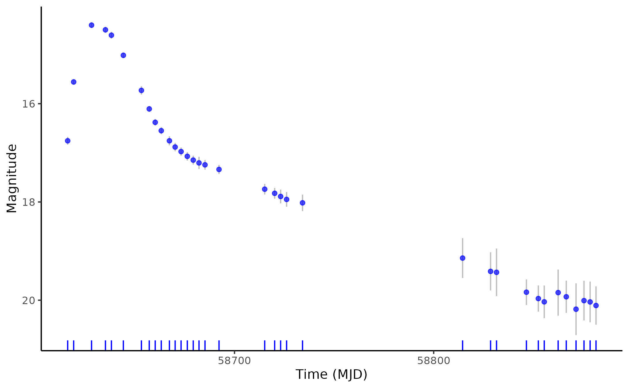
Treat the varying brightness of a source as a stochastic process
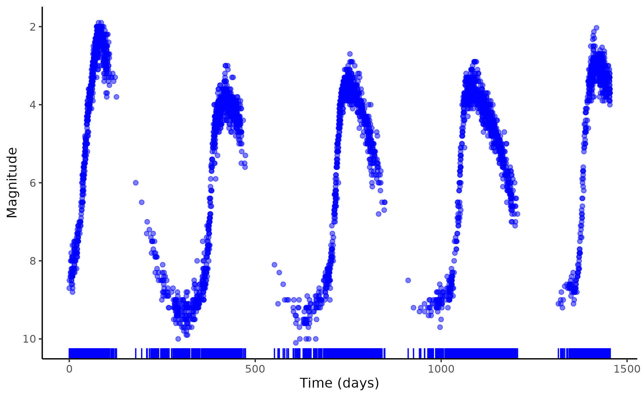
Magnitude
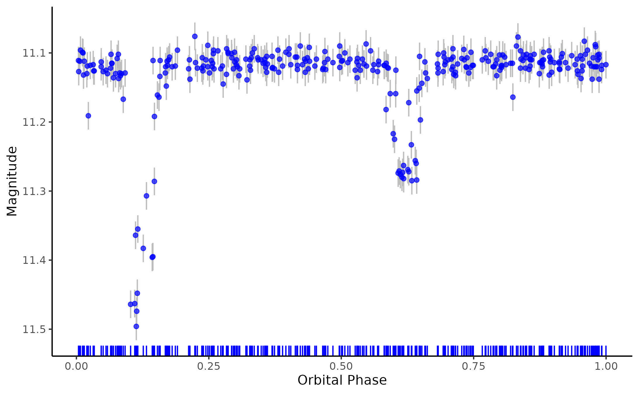
Magnitude
Magnitude
Time (days)
Orbital Phase
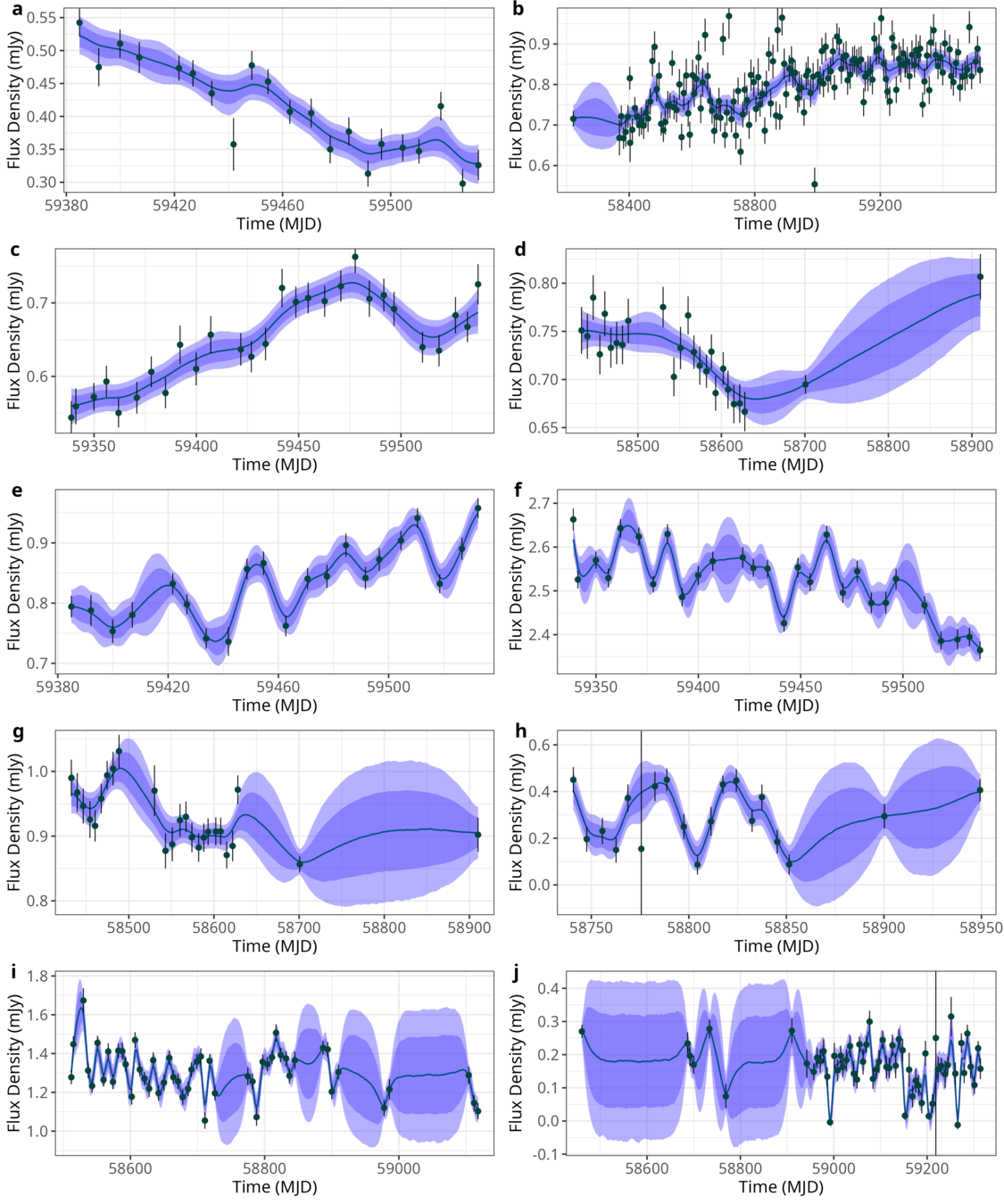
Time (MJD)
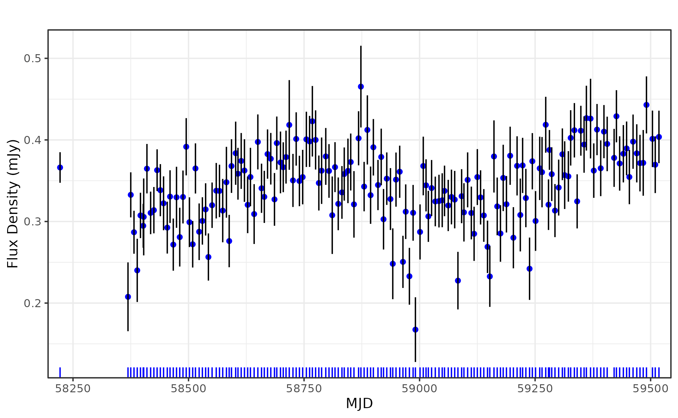
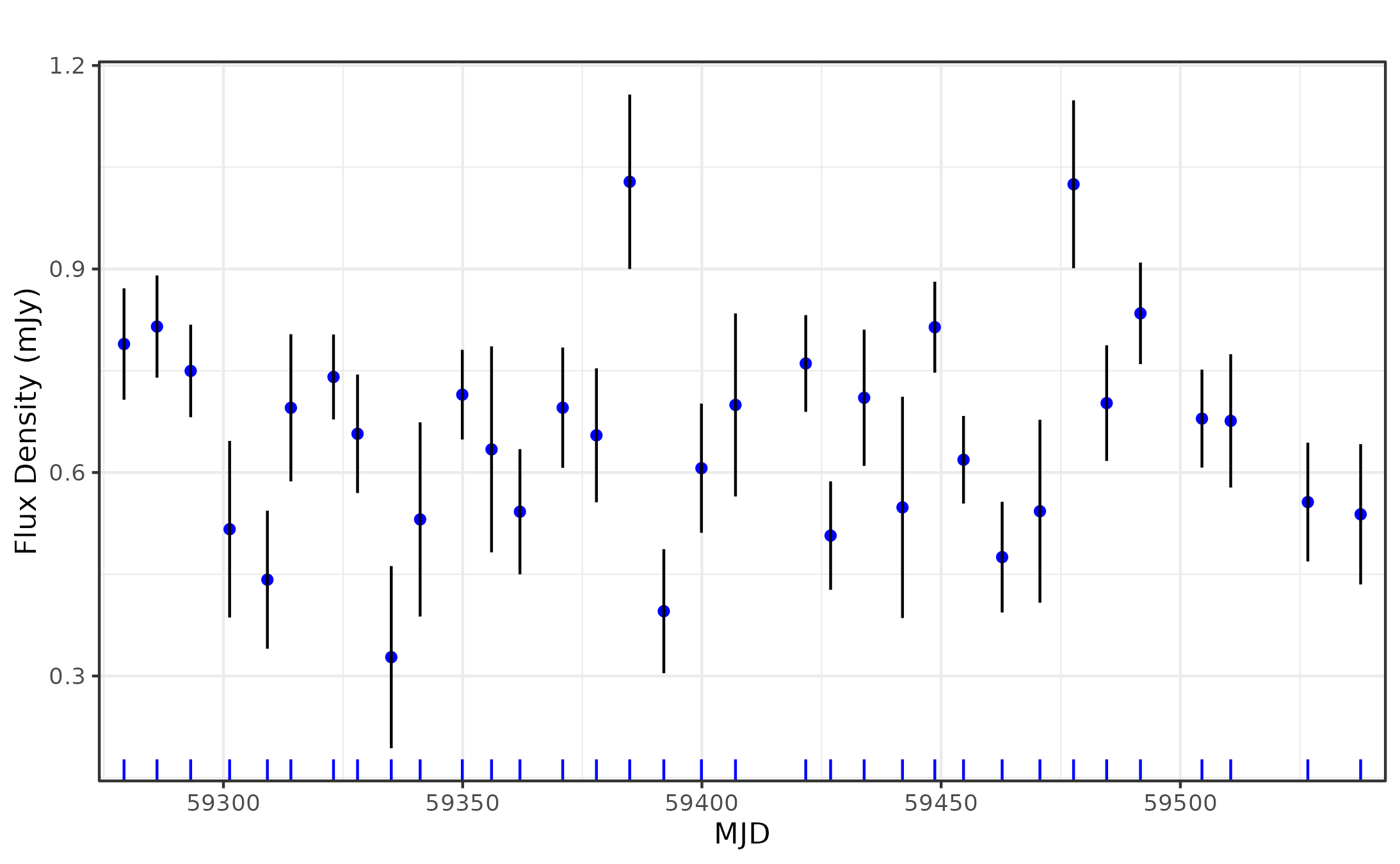
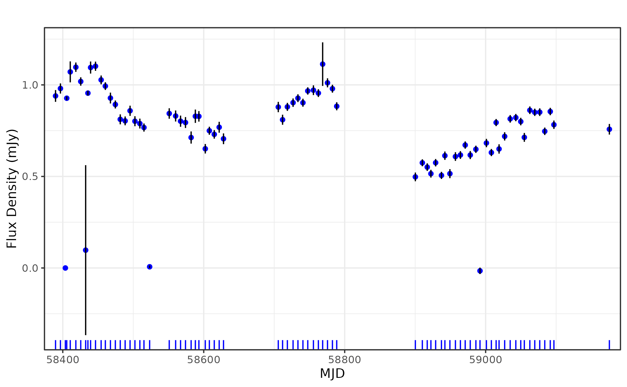
Heterogeneous Data
- Different cadences
- Sparse observations
- Uneven sampling rates
- Varying noise levels
Characterising Light Curves
- Fewer parameters
- Scales easily
- High information loss
- Many parameters
- High discriminatory power
- Overfitting
Oversimplified
Overspecified
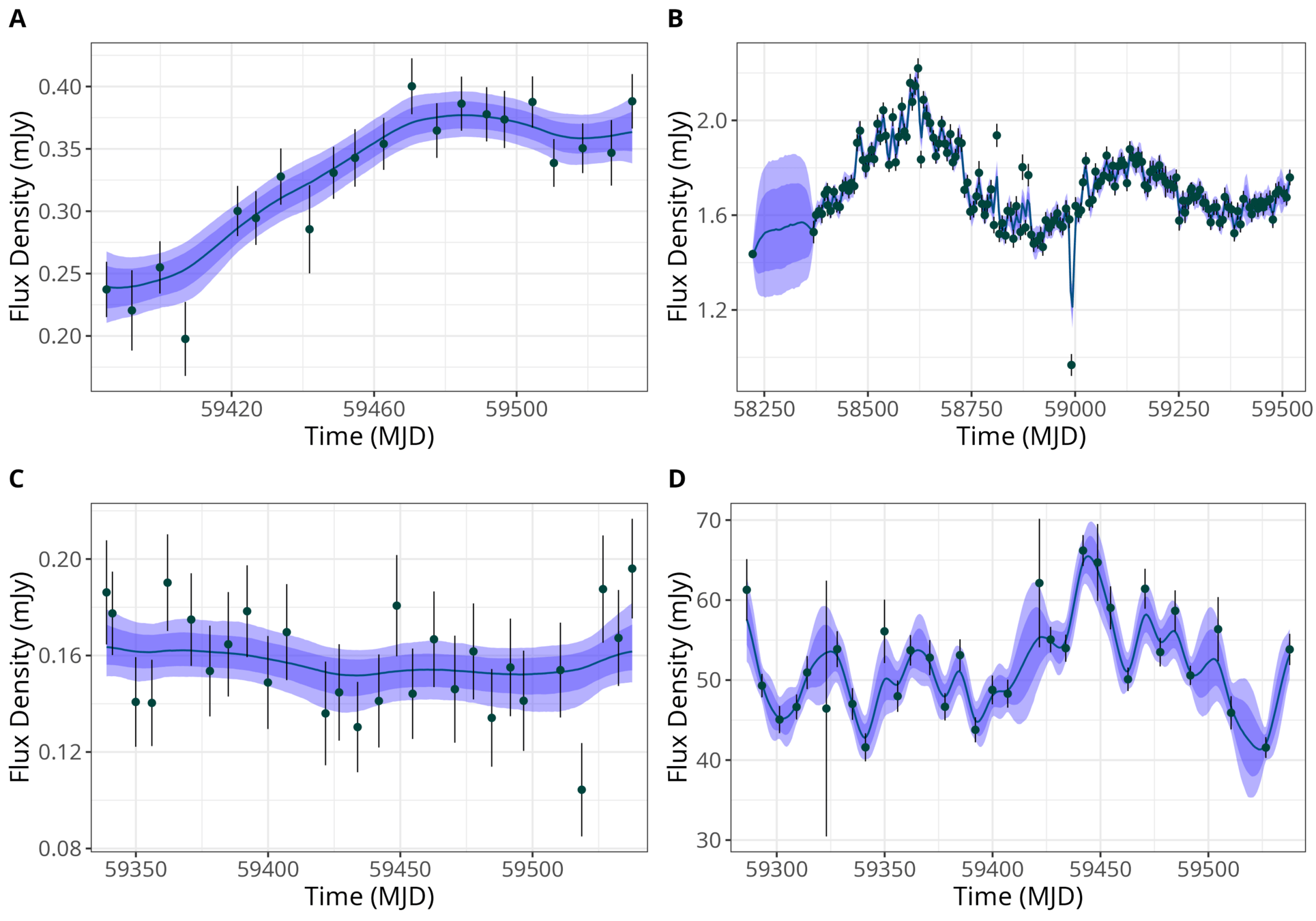
Model light curves as a Gaussian Process (GP)
Multivariate Normal
Y is a vector of n Gaussian distributed random variables.
where \(\boldsymbol\mu = (\mu_1, \dots, \mu_n)\) and \(\boldsymbol{\Sigma}\) is a \(n \times n \) covariance matrix.

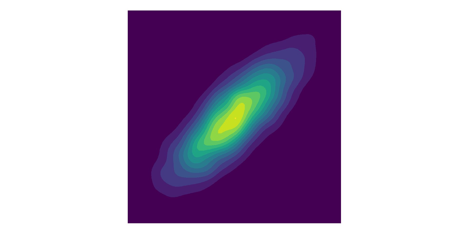
- Symmetric, positive semi-definite matrix.
- Linear combinations are also valid covariance matrices.
Gaussian Processes (GPs)
Extend multivariate Gaussian to 'infinite' dimensions.
- Mean function, \(\mu(t)\)
- Covariance or kernel function, \( \kappa(t,t') \)
where \(\mu = \mu(t_i)\) and \( [\boldsymbol\Sigma]_{ij} = \kappa(t_i, t_j) \), for \( i,j = 1, 2, \dots \)
Rather than specify a fixed covariance matrix with fixed dimensions, compute covariances using the kernel function.
Kernel Functions
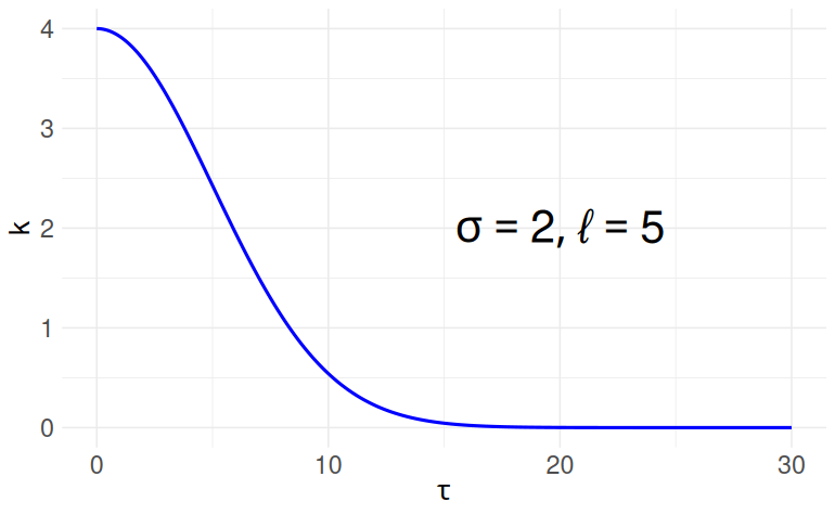
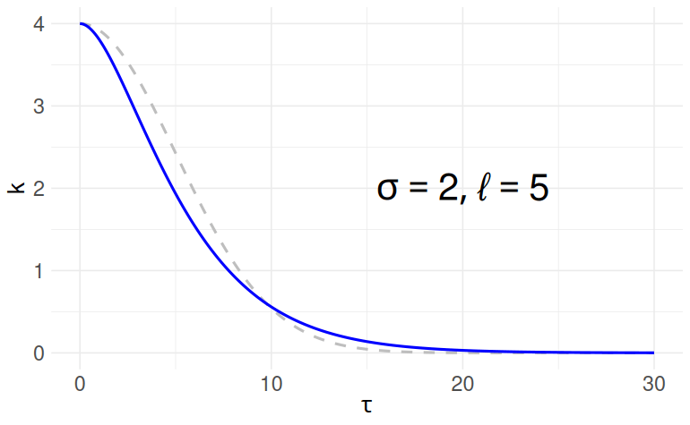
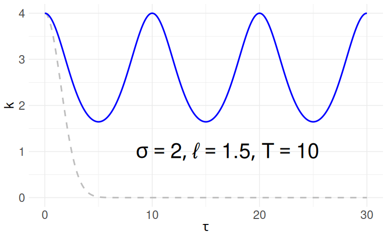
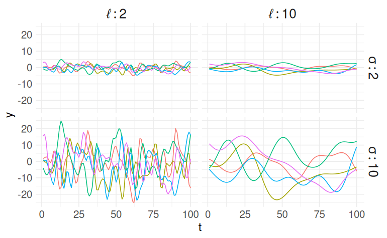
Squared Exponential
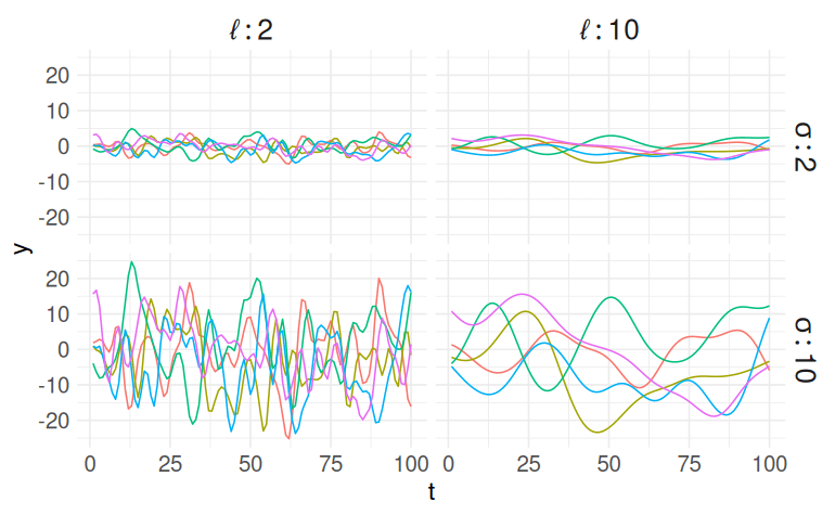
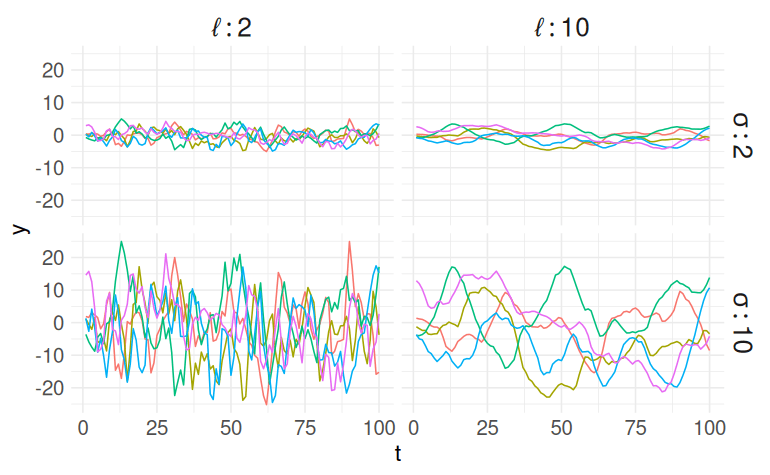
Matern 3/2
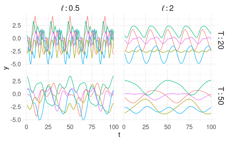
Periodic
$$\kappa(\tau; \sigma, \ell) = \sigma^2 \exp\left\{ -\frac{1}{2}\left( \frac{\tau}{\ell}\right)^2\right\}$$
$$\kappa(\tau; \sigma, \ell) = \sigma^2 \left( 1 + \sqrt{3}\frac{\tau}{\ell}\right) \exp\left\{ - \sqrt{3} \frac{\tau}{\ell}\right\}$$
$$\kappa(\tau; \sigma, \ell, T) = \sigma^2 \exp\left\{ -\frac{2}{\ell^2} \sin^2\left( \pi \frac{\tau}{T}\right)\right\}$$
Squared Exponential Kernel
Bayesian Hierarchical Model
Squared Exponential
Matern 3/2
Periodic
\(S_i \sim \mathcal{N}\left(f_i, \hat{e_i}^2\right)\)
\(\boldsymbol{f} \sim \mathcal{GP}\left(\boldsymbol{0}, \boldsymbol{\Sigma}_{n \times n}\right)\)
Hyperparameters
Flux density
GP prior
Bayesian Hierarchical Model
Data model
Process model
Parameter model
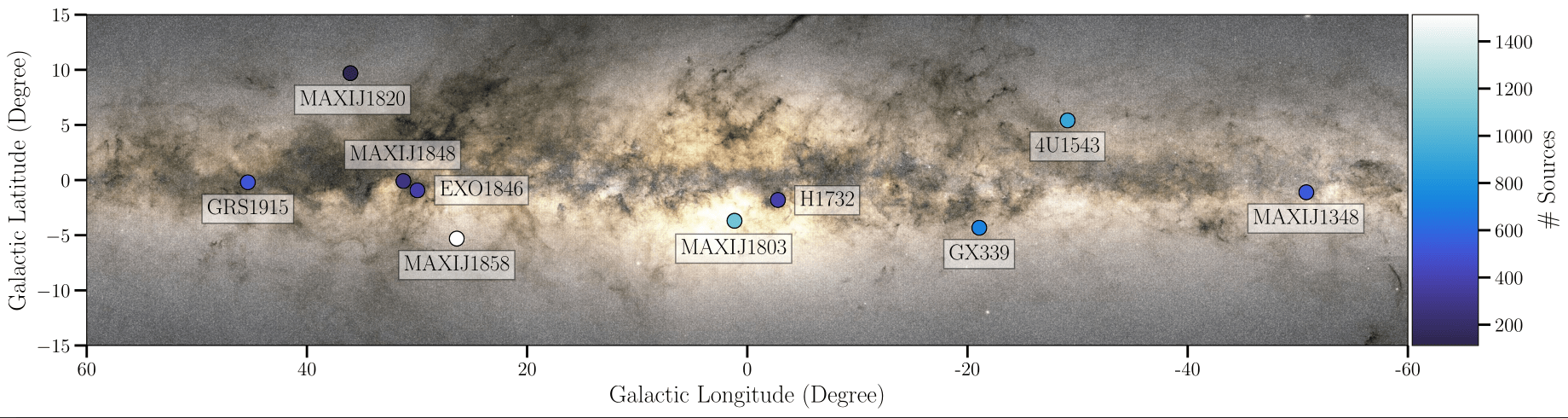
ThunderKAT Survey
- MeerKAT image domain transients survey
- Field-of-view of \(\approx 1^\circ \)
- 5,371 radio live curves over 10 fields
- Flux density and standard errors
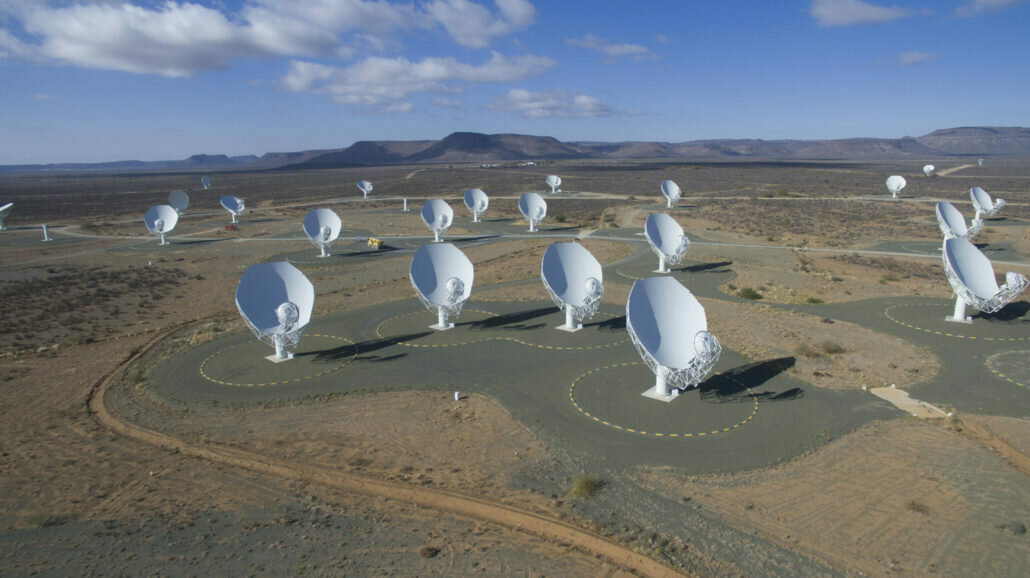
MeerKAT (Source: SARAO)
7D Hyperparameterspace
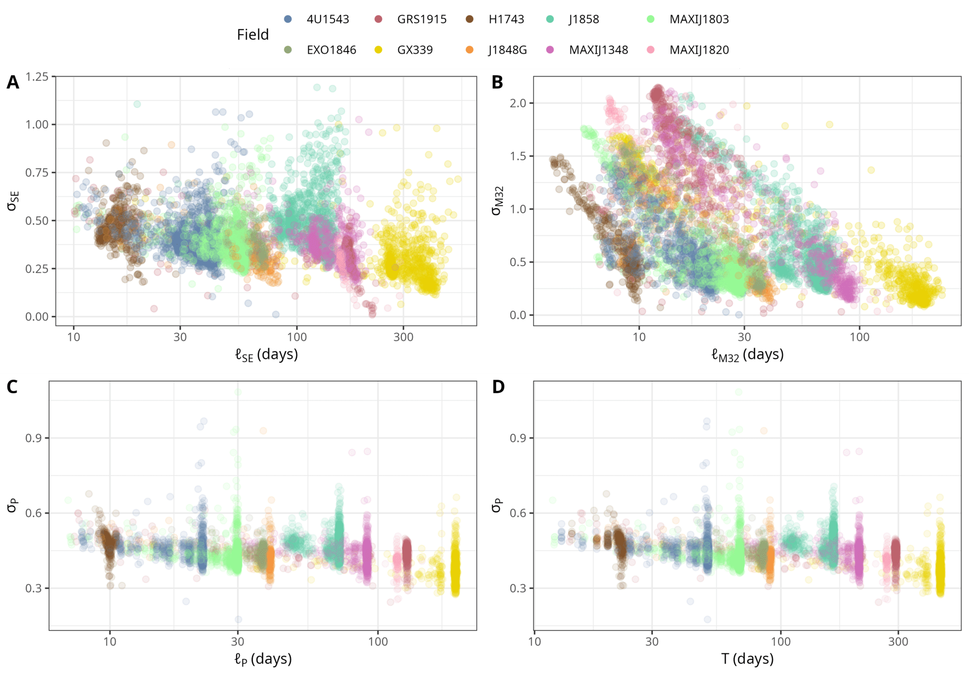
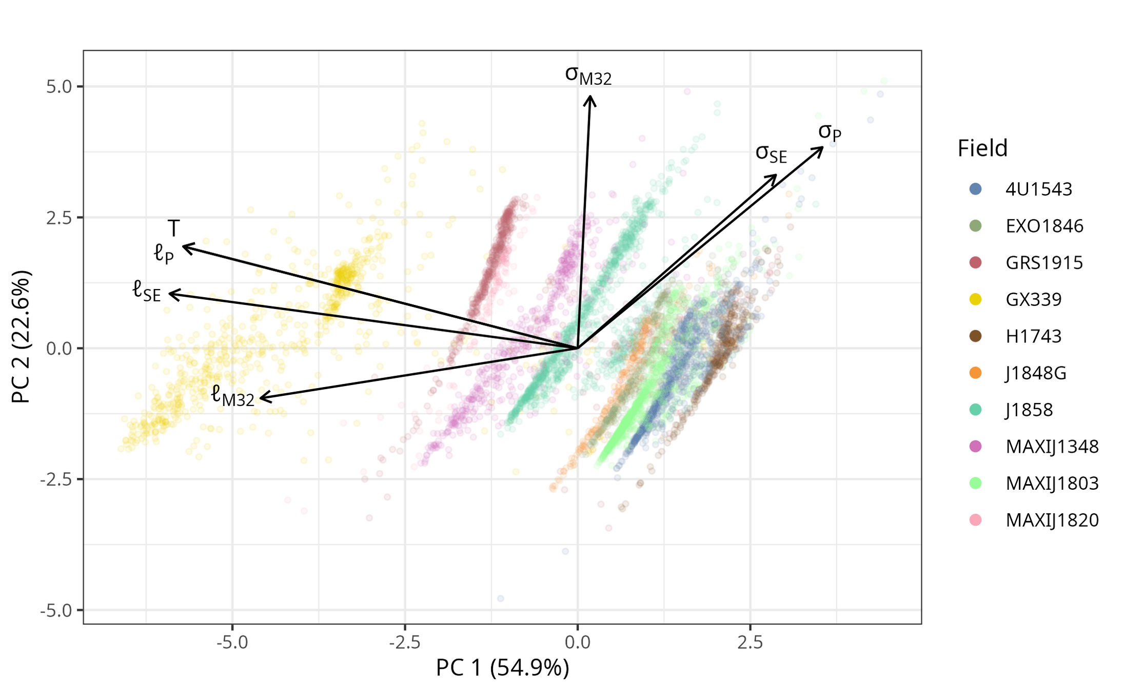
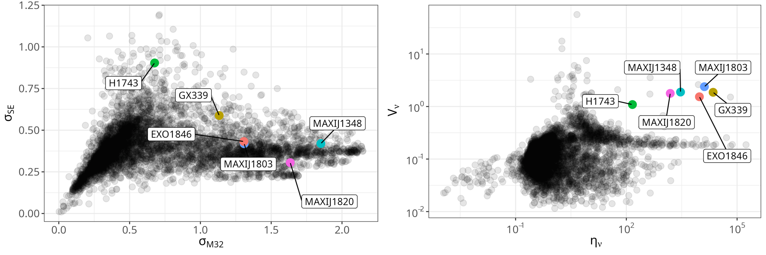
Amplitude Hyperparameters
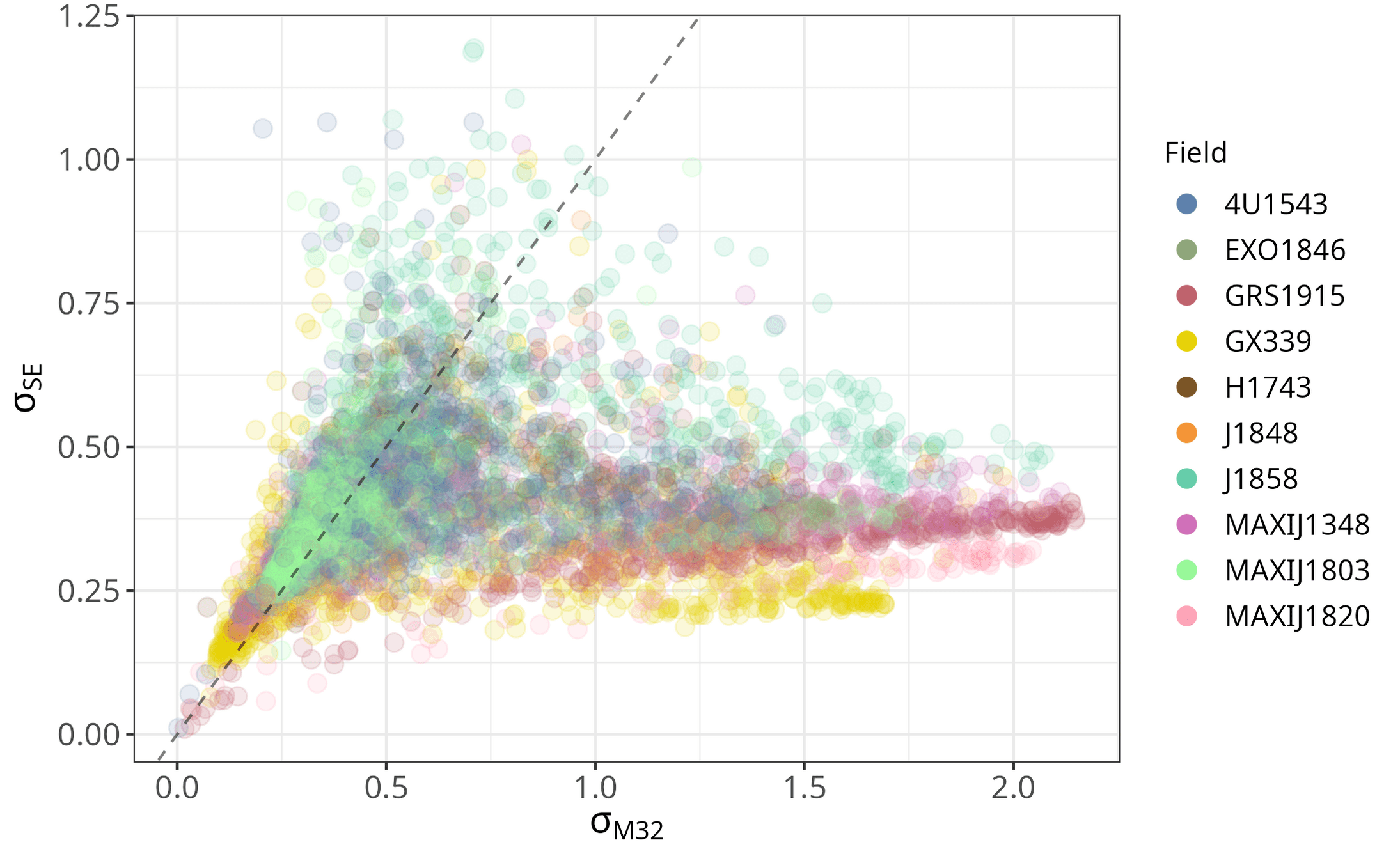
Interpeting Amplitude as Transience
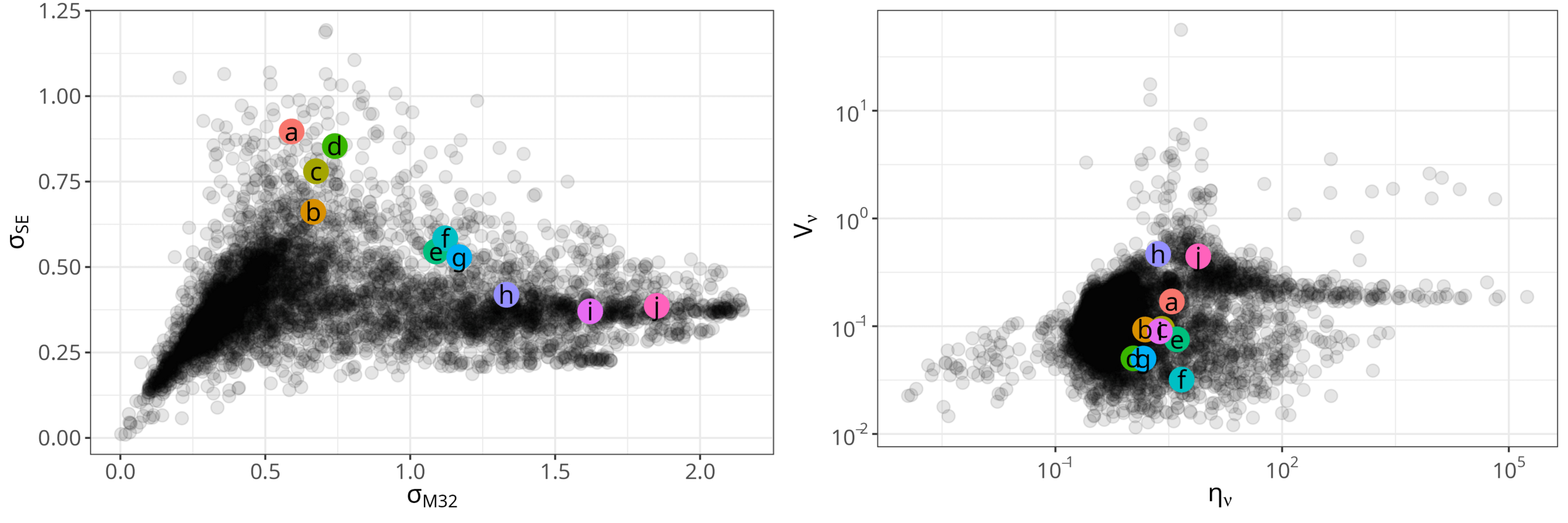
- Transience seems to manifest as large values in amplitude, \(\sigma_\mathrm{SE}\), \(\sigma_\mathrm{M32}\).
- Previously identified transient and variable candidates by Andersson et al. (2023) all seem to lie in the upper right of this 2D hyperparameter subspace.
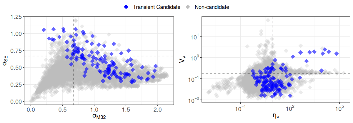
Data: Andersson et al. (2023)
Figure: Fu et al. (under review)
\( (\eta_\nu, V_\nu) \) vs. \( (\sigma_\mathrm{M32}, \sigma_\mathrm{SE})\)
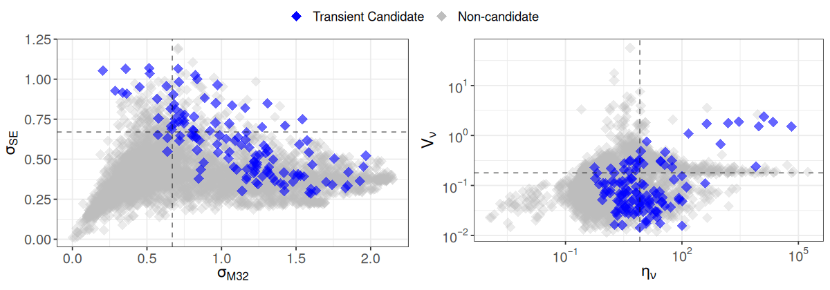
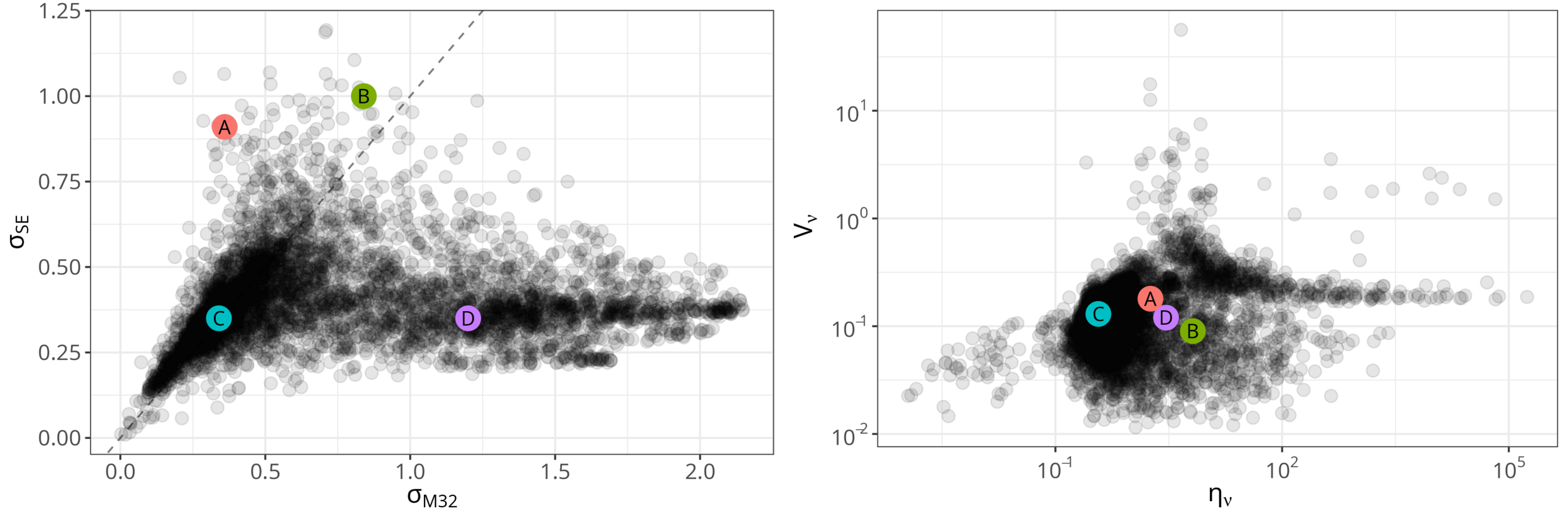
Parameterspace
\( (\eta_\nu, V_\nu) \) vs. \( (\sigma_\mathrm{M32}, \sigma_\mathrm{SE})\)
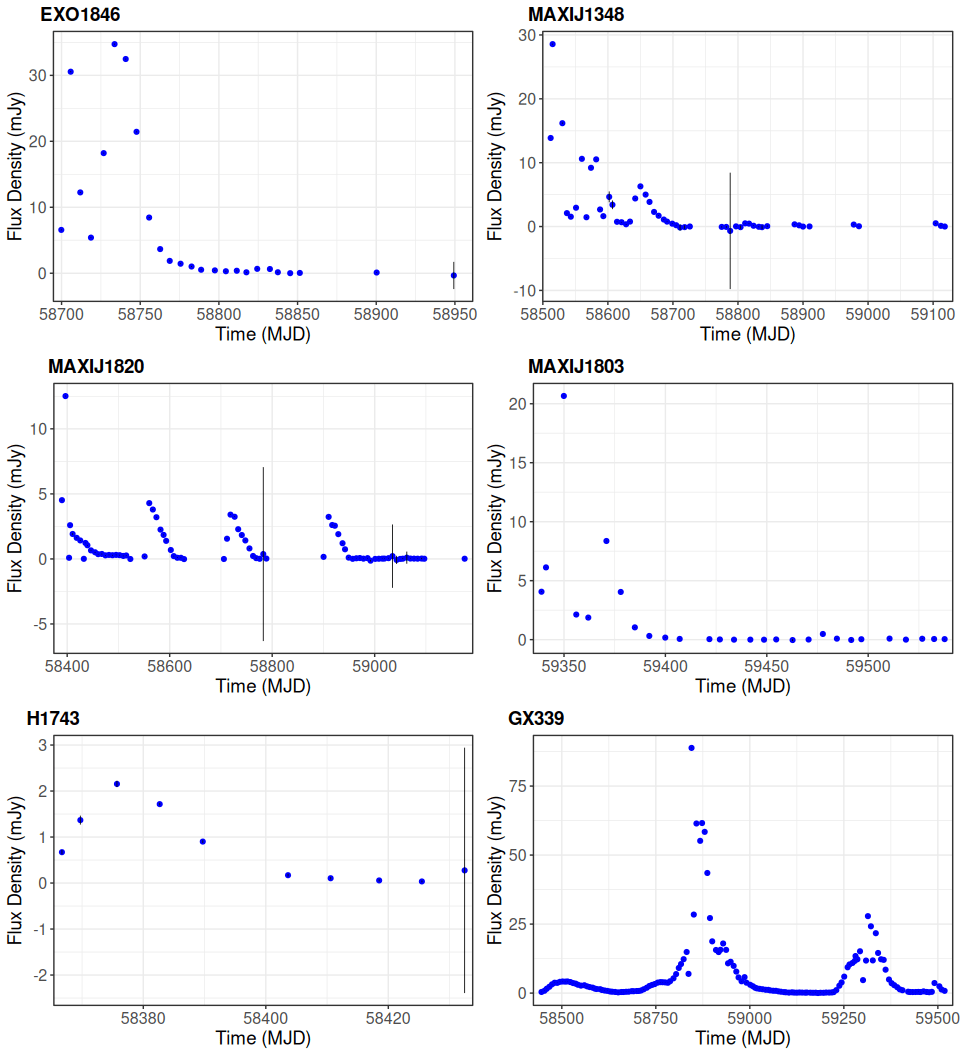
NN Candidates