COMP333 Algorithm Theory and Design - W1 2019

COMP333

Algorithm Theory and Design

Daniel Sutantyo

Department of Computing

Macquarie University

Lecture slides adapted from lectures given by Frank Cassez, Mark Dras, and Bernard Mans

Introduction

Unit Guide
- Unit Description
- Topics
- Assessment
- Textbook
Workshop + Code Repository

Problems and Algorithms

Computational Problems

A computational problem specifies the desired relationship between a set of values known as the input and a set of values known as the output
Examples:
- Given an array of integers $A$, find the largest value in the array $A$
- Given a positive integer $n$, find the nontrivial prime factors of $n$
- Given a map with $n$ cities and the cost of travelling between each pair of cities, find the cheapest way of travelling between city A and city B

Computational problems

A computational problem should have a well-defined input (including any constraints) and a well-defined output (and how it relates to the input)
Example:
- Given a positive integer $n$, find the nontrivial prime factors of $n$.
  - input: a positive integer $n$
  - output: the nontrivial prime factors of $n$
A particular input to a problem is referred to as an instance of a problem
- e.g. $n = 15$

Computational Problems

Given a map with $n$ cities and the cost of travelling between each pair of cities, find the cheapest way of travelling between city A and city B
- input:
  - a map with $n$ cities
  - the cost of travelling between any two cities
  - cities A and B
- output:
  - the cheapest way of travelling between city A and city B

Computational Problems

Given a positive integer $n$, find the nontrivial prime factors of $n$

...

[2]

[3]

...

[3,5]

...

"A computational problem can be viewed as an infinite collection of instances together with a solution for every instance." - https://en.wikipedia.org/wiki/Computational_problem

input

output

Computational Problems

These are not computational problems:
- Find the best place in Australia
  - what is a place? a city? a beach? a bar?
  - what does 'best' mean? how can we use the input to satisfy the output?
- Given a set of triangles, sort them
  - sort them according to what?

Types of Computational Problems

Decision problem: the output to every instance of input is either a yes or a no
- Given a positive integer $n$, is it a prime number?
- Given a map with $n$ cities and the cost of travelling between each city, can you travel from city A to city B for less than $x$?
Search problem: find one or more output that satisfies the required relation to the input
- Given a positive integer $n$, find its nontrivial prime factors
- Given a map with $n$ cities and the cost of travelling between each pair of cities, find all possible paths between city A and city B

Types of Computational Problems

Counting problem: find the number of solutions to a given search problem
- Given a positive integer $n$, how many nontrivial prime factors does it have?
- Given a map with $n$ cities and the cost of travelling between each pair of cities, find the number of possible paths between City A and City B
Optimisation problem: find the best possible solution among the set of all possible solutions to a search problem
- Given a map with $n$ cities and the cost of travelling between each pair of cities, find the cheapest cost of travelling between City A and City B

Algorithm

An algorithm is a computational procedure to solve a computational problem, i.e. to achieve the required relationship between the input and its output
An algorithm is correct if for every input instance, it halts with the correct output. If an algorithm is correct, it solves the given computational problem

Algorithm

The two most important aspects of algorithms that we are going to study in Comp333 are:
- Efficiency (complexity analysis)
- Correctness (algorithm design)
In the first two weeks we will discuss these two topics in more general terms, then we will revisit them as we discuss different types of algorithms, including:
- brute-force algorithms
- dynamic-programming algorithms
- greedy algorithms
- divide-and-conquer algorithms
- graph algorithms

Algorithm

Complexity analysis of algorithms

Correctness analysis of algorithms

Learn how to write efficient algorithms

Learn how to write correct algorithms

Learn how to design good algorithms

Why study algorithms?

Obvious solutions are not always tractable.
- tractable: can be solved in polynomial time, i.e. 'easy'
Tractable solutions can be improved
Recognise hard problems
- prevents us from wasting time looking for an efficient solution

Why study algorithms?

Obvious solutions are not always tractable

Problem:
- Given a map with $n$ cities and the cost of travelling between each pair of cities, find the cheapest way of travelling between city A and city B
Brute-force solution:
- Compute every single possible paths

Why study algorithms?

Obvious solutions are not always tractable

Brute-force solution:
- Compute every single possible paths
What is the number of possible paths from A to B?

no intermediate cities

1 intermediate city

$(n-2)$ choices

$\vdots$

2 intermediate cities

$(n-2)(n-3)$ choices

1 choice

Why study algorithms?

Obvious solutions are not always tractable

$$ 1 + (n-2) + (n-3)(n-2) + (n-4)(n-3)(n-2) + \cdots + \binom{n-2}{k}k! $$

Total number of paths:

(via 1 city)

(via 2 cities)

(via 3 cities)

(via $k$ cities)

For large $n$, it is impossible to check all paths, e.g. $50!\approx 3.04 \times 10^{64}$

Why study algorithms?

Obvious solutions are not always tractable

To be precise:

50! = 30,414,093,201,713,378,043,612,608,166,064,768,844,377,641,568,960,512,000,000,000,000

Can you think of a better way to find the shortest path?

Can you think of a better way to find the shortest path?

Why study algorithms?

Tractable solutions can be improved

Given a list of $n$ integers, find the largest and smallest integers among them
What is the minimum number of comparisons that you need to do?

$(n-1)$ comparisons, why?

How many comparisons do you need to find the largest and the smallest integers?

Why study algorithms?

Tractable solutions can be improved

Our first solution is likely to be $(2n-2)$ comparisons, i.e. just go through each numbers and record the maximum and minimum so far

We need $(2 * 8 - 2)$ = 14 comparisons in the above example

Our first solution is likely to be $(2n-2)$ comparisons, i.e. just go through each numbers and record the maximum and minimum so far

Why study algorithms?

Tractable solutions can be improved

Another method: (assume $n$ is even) pair up the numbers by doing $n/2$ comparisons

4 comparisons

3 comparisons

In total, the number of comparisons you need is roughly: $$\frac{n}{2} + \left(\frac{n}{2}-1\right) + \left(\frac{n}{2}-1\right) = \left(\frac{3n}{2} - 2\right)$$

Why study algorithms?

Recognise hard problems

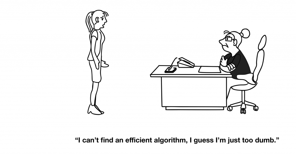
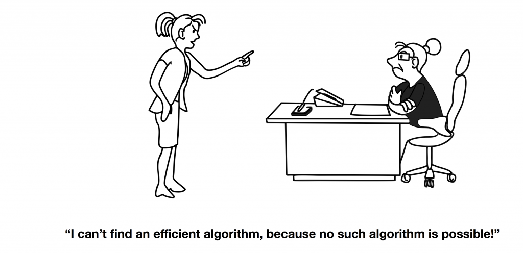
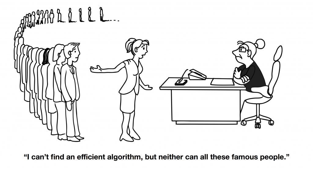
In later weeks you are going to learn about intractable problems, these are problems in which no polynomial (i.e. efficient) solutions are known
If you have to solve a problem, and you can see that it is intractable, then you should not waste time trying to find an efficient solution for it!

Cartoon by Stefan Szeider, available at https://www.ac.tuwien.ac.at/people/szeider/cartoon/

Why study algorithms?

Recognise hard problems

Cartoon by Stefan Szeider, available at https://www.ac.tuwien.ac.at/people/szeider/cartoon/

Why study algorithms?

Recognise hard problems

Cartoon by Stefan Szeider, available at https://www.ac.tuwien.ac.at/people/szeider/cartoon/

Why study algorithms?

Recognise hard problems

How do you study algorithms?

We start by going through the theoretical foundations
- so far we have defined a few terms which we will need for later parts (problems, intractability)
- later we will learn more tools (asymptotic notations, loop invariants)
We go through the most common problem solving strategies (divide-and-conquer, dynamic programming)
You learn by examples, and most importantly, by writing your own solutions

How do you study algorithms?

What makes a good chef?
- do you copy (or adapt) other people recipes?
- do you memorise recipes?
- do you only study recipes?
  - do you study the ingredients?
  - do you study your utensils?
- can you be a good chef if you only read and memorise recipes?
- can you be a good chef if you hardly ever cook?

Section Summary

Problem vs Algorithm
- input, constraint, output
- efficiency, correctness
- decision vs optimisation problem
Why study algorithms:
- to learn how to write better algorithms
- to recognise intractable problems

Complexity Analysis of Algorithms

RAM model of computation

Algorithm analysis should be language-independent and machine-independent
In other words you generally should not assume the use of a computer or programming language that can do complex operations quickly (e.g. factorisation, exponentiation)
It doesn't matter if your computer becomes 100 times faster, the complexity of the algorithm does not change. You do not measure the complexity of an algorithm using a stopwatch!

RAM model of computation

To analyse algorithms, we use a hypothetical simple computer called the Random Access Machine or RAM
Properties of RAM:
- we have primitive operations that take one time step each:
  - $+$ , $ -$ , $*$ , $\div$ , function calls, logical tests ($<$, $=$, $>$, etc)
- loops and subroutines are compositions of simple operations
- memory is unlimited and each memory access takes one time step
- instructions are executed one after another, i.e. no concurrency

RAM model of computation

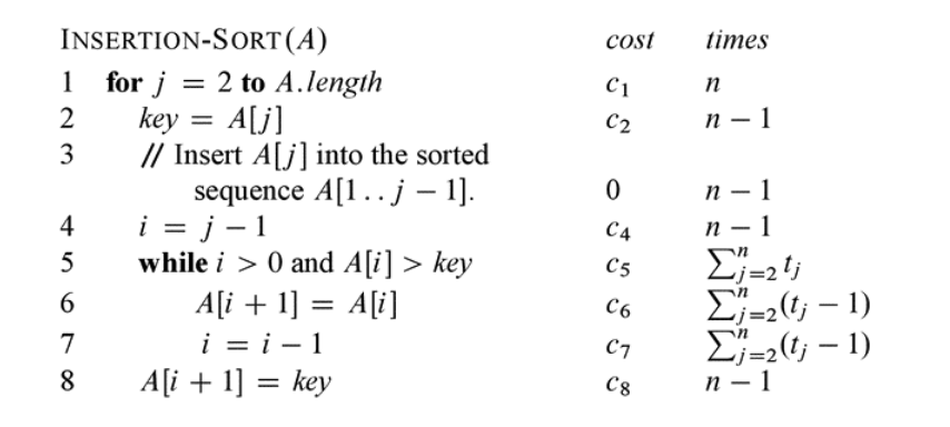
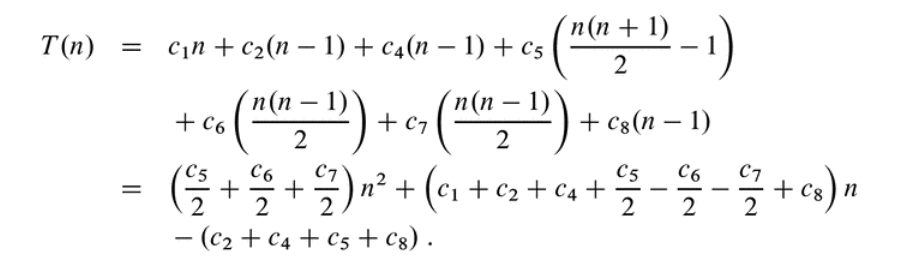
The running time or time complexity of an algorithm is the number of primitive operations that is executed by the algorithm
For a rigorous example, see CLRS pg 25- 27

RAM model of computation

Time complexity (or just complexity) of an algorithm is usually represented with the notation $T(n)$
The good (?) news is that in this unit, we are not going to do something as rigorous as what you saw in the previous slide
In most cases, it is enough to identify the most significant operation to derive the complexity of the algorithm

Best, worst, and average case complexity

An algorithm can have different time complexity depending on the input
- Insertion sort:
  - what is the most significant operation?
  - what input gives the fastest running time?
  - what input gives the slowest running time?

Best, worst, and average case complexity

sorted

unsorted

sorted

unsorted

Best case:

Worst case:

sorted

unsorted

Best, worst, and average case complexity

There can be many different inputs of size $n$
Worst-case complexity:
- the longest running time for any input of size $n$
Best-case complexity:
- the fastest running time for any input of size $n$
Average-case complexity:
- the average running time for inputs of size $n$

Best, worst, and average case complexity

Skiena, Figure 2.2, page 35

Best, worst, and average case complexity

In practice, the worst-case complexity is the most useful measure, although average-case complexity can also be useful
In this unit (and previous ones, e.g. Comp225), we are more interested in worst-case complexity
Average-case complexity can be difficult to derive (need to use probability theory)
Best-case complexity is the least useful

$O$-notation

It is hard to obtain exact formula for an algorithm's time complexity

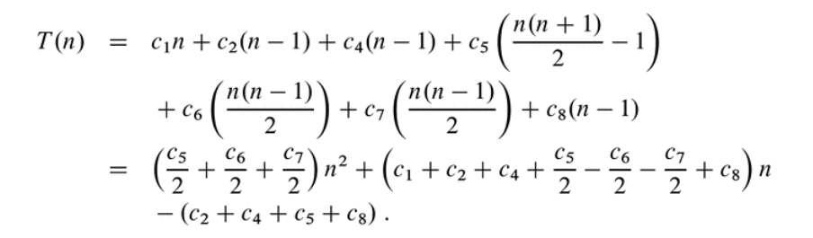
We can simplify this by ignoring constants and lower order terms
In computer science parlance, we a faster-growing function dominates a slower-growing one

$O$-notation

$n$ $n^2$ $n^{20}$ $2^n$ $2^{n+3}$

$100$

Dropping constants and lower-order terms does not impact our comparison of algorithms that much
- e.g. $2^{n+3} + 21n^{20} + 343n^2 + 1729n + 17013$

$200$

$1 \times 10^4$

$1 \times 10^{40}$

$1.26 \times 10^{30}$

note: $10^{40}$ is a ten billion times bigger than $10^{30}$

$4 \times 10^4$

$1.05 \times 10^{46}$

$1.61 \times 10^{60}$

$300$

$9 \times 10^4$

$3.49 \times 10^{49}$

$2.04 \times 10^{90}$

$400$

$1.6 \times 10^5$

$1.10 \times 10^{52}$

$2.58 \times 10^{120}$

$1.01 \times 10^{31}$

$1.28 \times 10^{61}$

$1.63 \times 10^{91}$

$2.07 \times 10^{121}$

$O$-notation

We use asymptotic notations (or asymptotic functions) to make it simpler for us to compare algorithms
One asymptotic notation you already know well, the $O$-notation, is the asymptotic upper bound
$f(n) = O(g(n))$ means there exists a constant $c$ such that for all $n > n_0$, $f(n) \le c\cdot g(n) $

$O$-notation

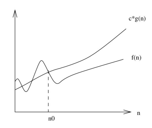
Skiena Figure 2.3, page 36

$f(n)$

$c\cdot g(n)$

$O$-notation

$f(n) = O(g(n))$ means there exists positive constants $c$ and $n_0$ such that for all $n > n_0$, $f(n) \le c\cdot g(n) $
example:
$ 3n^2 + 100n + 25 = O(n^2) $ because

$3n^2 + 100n + 25 \le 100n^2 + 100n^2 + 100n^2 = 300n^2$

i.e. use $c = 300$ and $n_0 = 1$

for all $n \ge 1$

(that wasn't hard to prove, was it?)

for all $n \ge 1$

$O$-notation

Remember, $O$-notation is a method to express the complexity of an algorithm
- You can express an algorithm's worst-case complexity using $O$-notation
- You can express an algorithm's average-case complexity using $O$-notation
- You can express an algorithm's best-case complexity using $O$-notation
You simply use $O$-notation is to denote the upper bound for the best/average/worst case complexity of an algorithm!

Remember, $O$-notation is a method to express the complexity of an algorithm
- You can express an algorithm's worst-case complexity using $O$-notation
- You can express an algorithm's average-case complexity using $O$-notation
- You can express an algorithm's best-case complexity using $O$-notation
You simply use $O$-notation is to denote the upper bound for the best/average/worst case complexity of an algorithm!

$O$-notation

Asymptotic analysis studies how the algorithm behaves as $n$ tends to infinity
We ignore lower order terms and constants because as $n$ tends to infinity, these become insignificant
We ignore constant multipliers because the growth rate is more important
By ignoring these usually unimportant details, we obtain a representation that succinctly describes the growth of a function and can thus make comparisons between algorithms more easily

$O$-notation

Questions:
- is $n^2 + 1000n = O(n)$?
- is $n = O(n^2)$?
- is $2^{n+1} = O(2^n)$?
- is $2^{2n} = O(2^n)$? (will be a workshop question)

$\Omega$-notation

$\Omega$-notation is the asymptotic lower bound
$f(n) = \Omega(g(n))$ means there exists positive constants $c$ and $n_0$ such that for all $n > n_0$, $f(n) \ge c\cdot g(n) \ge 0$

$\Omega$-notation

Skiena Figure 2.3, page 36

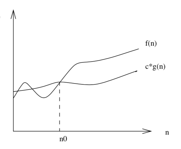
$c\cdot g(n)$

$ f(n)$

$\Theta$-notation

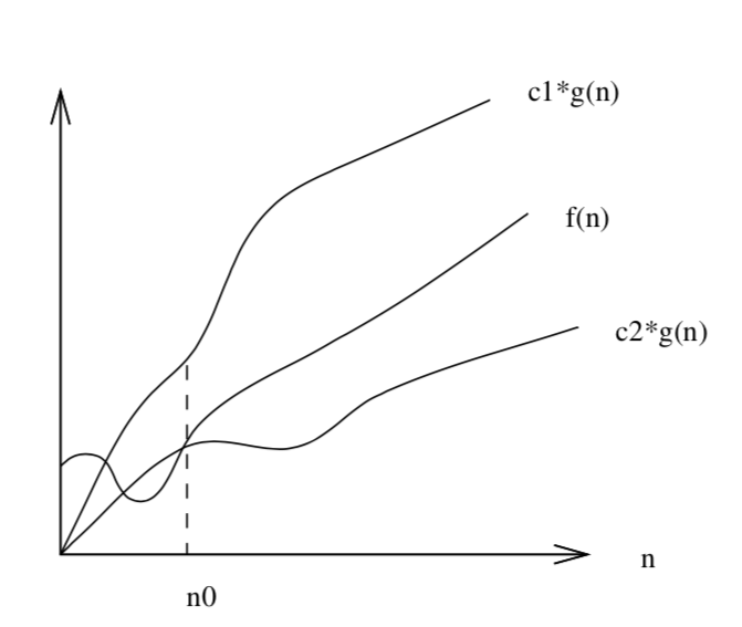
$\Theta$-notation is the asymptotic tight bound
$f(n) = \Theta(g(n))$ means there exists positive constants $c_1$, $c_2$, and $n_0$ such that for all $n > n_0$,
$0 \le c_1\cdot g(n) \le f(n) \le c_2\cdot g(n) $
$f(n) = \Theta(g(n))$ if and only if $f(n) = \Omega(g(n))$ and $f(n) = O(g(n))$

$\Theta$-notation

Skiena Figure 2.3, page 36

$f(n)$

$c_2\cdot g(n)$

$c_1\cdot g(n)$

Addendum

worst-case vs average-case

Which one is more useful, worst-case complexity or average-case complexity?
- it really depends on what the goal of the analysis is
  - worst-case analysis can be too pessimistic
  - average-case analysis can be too optimistic
  - (aside: can you think of a use for best-case analysis?)
- average-case complexity is usually harder to derive:
  - what is your average input?
- maybe worst-case complexity is 'good enough'

Addendum

asymptotic notation

We often use $O$-notation to describe a tight bound, i.e. we use $O$-notation, when we really should be using $\Theta$-notation
Note that all of these are correct
- $2^n = O(2^n)$
- $n^2 = O(2^n)$
- $n = O(2^n)$
- $\log n = O(2^n)$
But are these useful?

Addendum

asymptotic notation

Remember, we are using asymptotic notation to describe, the running time of our algorithm.
How useful are these?
- $T(n) = O(2^n)$
- $T(n) = O(n^2)$
- $T(n) = O(n)$
- $T(n) = O(\log n)$
Even when you are using $O$-notation, you would want to describe the running time as accurately as possible

Addendum

asymptotic notation

Finally, remember that
- $f(n) = \Theta(g(n)) \implies f(n) = O(n)$
For many algorithms, we can find a tight bound for their time complexity, so in these cases there is little difference between using $\Theta(g(n))$ or $O(g(n))$

Recurrence

and
Induction

Recurrence and Induction

We will now briefly see how we can evaluate the running time of an algorithm
We will study this topic more deeply in later weeks, but it is good to start now to give you some intuition

Divide and Conquer Algorithm

A divide-and-conquer algorithm is an algorithm that breaks down the original problem into smaller and smaller subproblems and solve them recursively
Two examples of divide-and-conquer algorithms are binary search and merge sort
We can describe the running time of these algorithms using a recurrence equation (or just recurrence)

Divide and Conquer Algorithm

A recurrence equation describes the running time on a problem of size $n$ in terms of the running time on smaller inputs
Formally:

$T(n) = \begin{cases} \Theta(1) &\text{if $n \le c$}\\ aT(n/b) + D(n) + C(n) &\text{otherwise} \end{cases}$

where

$D(n)$ is the cost of dividing the problem into subproblems, and
$C(n)$ is the cost of combining solutions of the subproblems to create a solution for the problem

Divide and Conquer Algorithm

mergesort

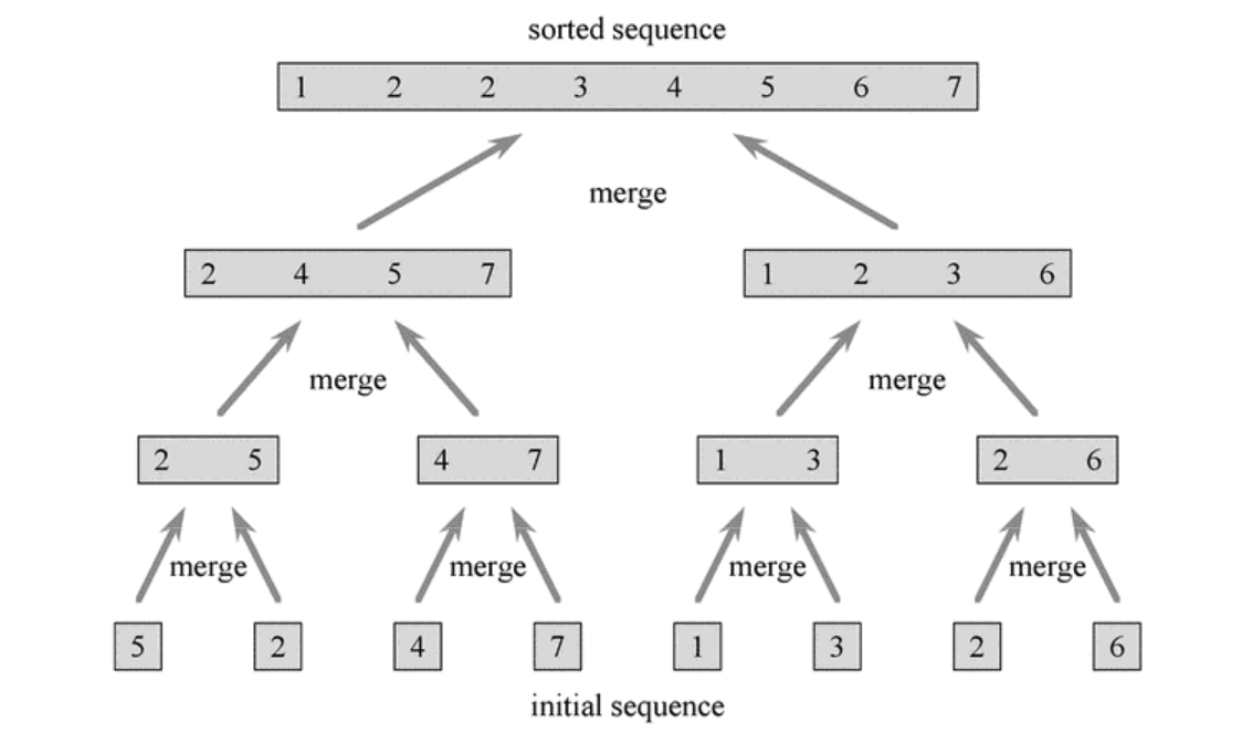
(from CLRS, Figure 2.4, page 35)

Divide and Conquer Algorithm

mergesort

The running time can be derived as follows:
- Divide: computes the middle of the subarray
  - $D(n) = \Theta(1)$
- Conquer: solve two subproblems of size $n/2$ each
  - $2T(n/2)$
- Combine: merging two subarrays of size $n/2$ each
  - $C(n) = \Theta(n)$
Therefore the running time of merge sort is

$T(n) = \begin{cases} \Theta(1) &\text{if $n = 1$}\\ 2T(n/2) + \Theta(n) &\text{if $n > 1$} \end{cases}$

Divide and Conquer Algorithm

mergesort

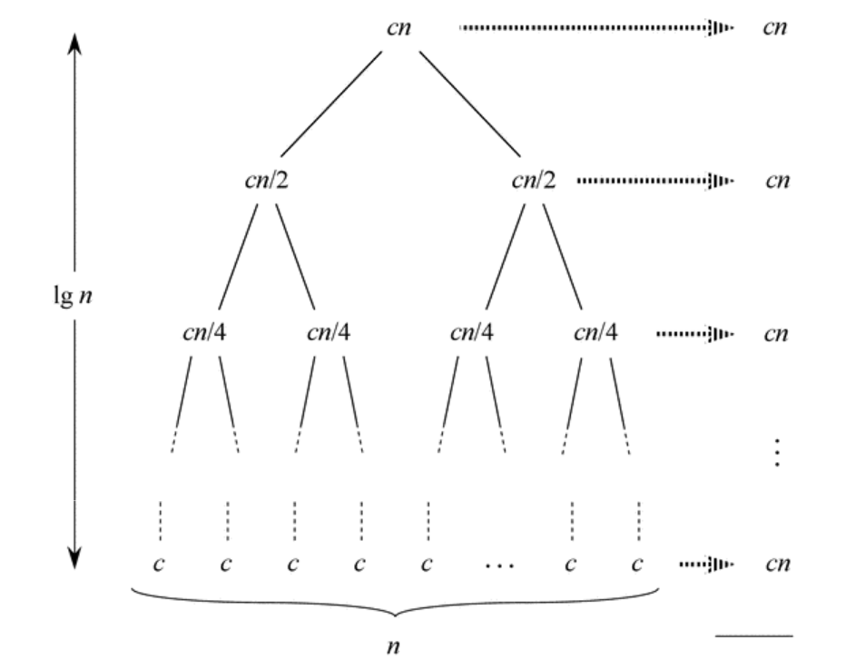
To work out the time complexity of merge sort, we can look at the recursion tree generated by this algorithm
Let us assume that it costs $c$ to solve a problem of size 1 and also $c$ to combine one array element

$T(n) = \begin{cases} \Theta(1) &\text{if $n = 1$}\\ 2T(n/2) + \Theta(n) &\text{if $n > 1$} \end{cases}$

$T(n) = \begin{cases} c &\text{if $n = 1$}\\ 2T(n/2) + cn &\text{if $n > 1$} \end{cases}$

Divide and Conquer Algorithm

mergesort

Divide and Conquer Algorithm

mergesort

There are $\log n$ levels, and on each level we need to perform $cn$ operations
Therefore merge sort is $\Theta(n\log n)$
... by the way, was that worst-case, average-case, or best-case?

Divide and Conquer Algorithm

binary search

$T(n) = \begin{cases} \Theta(1) &\text{if $n = 1$}\\ T(n/2) + \Theta(1) &\text{if $n > 1$} \end{cases}$

is this worst-case, average-case, or best-case?

Divide and Conquer Algorithm

binary search

$\log n$

so binary search is $\Theta(\log n)$

Divide and Conquer Algorithm

more recurrence equations

Sequential search:
- $T(n) = T(n-1) + O(1)$
Tree traversal:
- $T(n) = 2T(n/2)+O(1)$
Selection sort/Insertion sort
- $T(n) = T(n-1) + O(n)$

Divide and Conquer Algorithm

deriving time complexity

There are three main ways to derive the time complexity of a divide-and-conquer algorithm:
- using recursion-tree method
- using substitution method (requires proof by induction)
  - we will cover this in Week 6
- using master method (master theorem)

Divide and Conquer Algorithm

master theorem

Given a recurrence of the form
- $T(n) = aT(n/b) + f(n) $
if $f(n) = O(n^{\log_b a-\epsilon})$ for some constant $\epsilon > 0$
- then $T(n) =\Theta(n^{\log_b a})$
if $f(n) = \Theta(n^{\log_b a})$
- then $T(n) = \Theta(n^{\log_b a}\log n)$
if $f(n) = \Omega(n^{\log_b a + \epsilon})$ for some constant $\epsilon > 0$, and if $a f(n/b) \le cf(n)$ for some $c < 1$
- then $T(n) = \Theta(f(n))$

Divide and Conquer Algorithm

master theorem

Usage example:
- $T(n) = aT(n/b) + f(n) $
- if $f(n) = \Theta(n^{\log_b a})$
  - then $T(n) = \Theta(n^{\log_b a}\log n)$
- merge sort recurrence is $T(n) = 2T(n/2) + \Theta(n)$
  - $a = 2$, $b = 2$
  - thus merge sort is $\Theta(n\log n)$

Proof by induction

We are going to use proof by induction a few times in Comp333, so here is a quick refresher
If you need to revise proof by induction, you can refer to your DMTH237 Textbook: Discrete Mathematics and Its Applications (7th Edition) by Kenneth H. Rosen, Chapter 5
I also like How to Prove It: A Structured Approach by Daniel J. Velleman (highly recommended for revising your mathematics)

Proof by induction

Mathematical induction is used to prove that a certain statement holds (i.e. is true) for every natural number
- e.g. show that $\sum_{i=1}^n i = \frac{n(n+1)}{2}$ for all $n \in \mathbb N$
Informally, to prove something by induction, you show these two:
- show that the statement is true for $n=1$ (the base case)
- show that if the statement is true for $n=k$, then it is also true for $n = k +1$
If you can show these two, then the statement is true for all $n \ge 1$: If it's true for 1, then it's true for 2. If it's true for 2, then it's true for 3, and so on ...

Proof by induction

If you are asked to write a proof by induction in Comp333, you do need to write it formally
Your proof should have the following form:
- Base case: prove that the statement is true for $n = 1$ (or another value of $n$ as appropriate)
- Induction step:
  - induction hypothesis: assume that the statement is true for $n = k$, where $k \ge 1$, $k \in \mathbb N$
  - prove that if the statement is true for $n = k$, then it is also true for $n = k + 1$

Proof by induction

Show that
- Base case: show that the statement is true for $n=1$
  - if $n = 1$ then
  - LHS = RHS, thus the property is true for $n=1$

LHS :

\[ \sum_{i=1}^1 i = 1\]

\[\frac{1(1+1)}{2} = 1\]

RHS :

\[\sum_{i=1}^n i = \frac{n(n+1)}{2}\]

Proof by induction

Induction step
- induction hypothesis: assume that the statement is true for $n = k$, that is we assume

\[ \sum_{i=1}^k i = \frac{k(k+1)}{2} \text{for some $k \ge 1, k \in \mathbb N$}\]

Proof by induction

Induction step
- now we prove that if the property holds for $n =k$, then it also holds for $n =k+1$
- that is, we have to prove that
  \[ \sum_{i=1}^{k+1} i = \frac{(k+1)(k+2)}{2}\]

Remember, the statement we need to prove is

\[\sum_{i=1}^n i = \frac{n(n+1)}{2}\]

Proof by induction

Induction step:

\[\sum_{i=1}^{k+1} i = (k+1) + \sum_{i=1}^{k} i \]

\[= (k+1) + \frac{k(k+1)}{2} \]

\[= \frac{2k+2 + k^2 + k}{2} = \frac{k^2 +3k + 2}{2}\]

\[= \frac{(k+1)(k+2)}{2}\]

(as required)

(from the induction hypothesis)

Incorrect proof by induction

If you make the wrong induction hypothesis, i.e. you make the wrong assumption, then your proof will end up being wrong!
In other words, you can prove whatever you want using induction!
- No, not really ... but this is a common mistake in writing proofs by induction

Incorrect proof by induction

Show that

(from CLRS, Appendix A, page 1150)

Base case: if $n = 1$, obviously $1 = O(1)$
Induction step:
- induction hypothesis:
- want to show that:

\[\sum_{i=1}^n i = O(n) \]

\[\sum_{i=1}^{k+1} i = (k+1) + \sum_{i=1}^k i = O(k) + k+1 = O(k+1)\]

\[\sum_{i=1}^k i = O(k)\]

\[\sum_{i=1}^{k+1} i = O(k+1)\]

WRONG!

More examples

Show that

Base case: if $n = 1$
- LHS : $1 \times 1! = 1$
- RHS : $(1+1)! - 1 = 2 - 1 = 1$
- so LHS = RHS, the statement is true for $n = 1$

\[\sum_{i=1}^n (i \times i!) = (n+1)! - 1 \]

Induction step:
- assume true for $n = k$, i.e
- we need to prove that

\[\sum_{i=1}^k (i \times i!) = (k+1)! - 1 \]

\[\sum_{i=1}^{k+1} (i \times i!) = (k+2)! - 1 \]

More examples

\[\sum_{i=1}^{k+1} (i \times i!) = (k+1) \times (k+1)! + \sum_{i=1}^k (i \times i!) \]

\[= (k+1) \times (k+1)! + (k+1)! - 1\]

\[= (k+1)! ( k+1+1) - 1\]

\[= (k+2)(k+1)! - 1\]

\[= (k+2)! - 1\]

as required

More examples

Show that

Base case: if $n = 5$
- LHS : $2^5 = 32$
- RHS : $5^2 = 25$
- so LHS > RHS, the statement is true for $n = 5$

$2^n > n^2$ for $n \ge 5$

Induction step:
- assume true for $n = k$, $k \ge 5$ i.e. we assume $2^k > k^2$
- we need to prove that $2^{k+1} > (k+1)^2$

More examples

Induction step:
- assume true for $n = k \ge 5$ i.e. we assume $2^k > k^2$
- we need to prove that $2^{k+1} > (k+1)^2$

$2^{k+1} = 2\cdot 2^k > 2k^2 = k^2 + k^2 $

since $k \ge 5$, we have $k^2 \ge 5k$, hence

$2^{k+1} > k^2 + 5k > k^2 + 2k + 1 = (k+1)^2$

as required

More examples

Prove that a tree with $n$ vertices has $(n-1)$ edges
Base case:
- by inspection, we can see that
  - a tree with $1$ node has 0 edges,
  - a tree with $2$ nodes have 1 edge, and
  - a tree with $3$ nodes have 2 edges
Induction step:
- assume true for $n = k$, that is, a tree with $k$ vertices have $(k-1)$ edges
- can we show that this is also true for $n=k+1$ ?

More examples

Induction step:
- we assume a tree with $k$ vertices have $(k-1)$ edges
- we need to show that a tree with $(k+1)$ vertices has $k$ edges
  - any tree with $(k+1)$ vertices must have one vertex that has degree 1 (why?)
  - if we remove the vertex with degree 1 (and the edge connecting it), we will end up with a tree with $k$ vertices, and by our assumption, this tree has $(k-1)$ edges
  - thus a tree with $(k+1)$ vertices has $k$ edges

COMP333

Algorithm Theory and Design

Lecture slides adapted from lectures given by Frank Cassez, Mark Dras, and Bernard Mans

Introduction

Problems and Algorithms

Computational Problems

Computational problems

Computational Problems

Computational Problems

Computational Problems

Types of Computational Problems

Types of Computational Problems

Algorithm

Algorithm

Algorithm

Why study algorithms?

Why study algorithms?

Obvious solutions are not always tractable

Why study algorithms?

Obvious solutions are not always tractable

Why study algorithms?

Obvious solutions are not always tractable

Why study algorithms?

Obvious solutions are not always tractable

Why study algorithms?

Tractable solutions can be improved

Why study algorithms?

Tractable solutions can be improved

Why study algorithms?

Tractable solutions can be improved

Why study algorithms?

Recognise hard problems

Why study algorithms?

Recognise hard problems

Why study algorithms?

Recognise hard problems

Why study algorithms?

Recognise hard problems

How do you study algorithms?

How do you study algorithms?

Section Summary

Complexity Analysis of Algorithms

RAM model of computation

RAM model of computation

RAM model of computation

RAM model of computation

Best, worst, and average case complexity

Best, worst, and average case complexity

Best, worst, and average case complexity

Best, worst, and average case complexity

Best, worst, and average case complexity

\(O\)-notation

\(O\)-notation

\(O\)-notation

\(O\)-notation

\(O\)-notation

\(O\)-notation

\(O\)-notation

\(O\)-notation

\(\Omega\)-notation

\(\Omega\)-notation

\(\Theta\)-notation

\(\Theta\)-notation

Addendum

worst-case vs average-case

Addendum

asymptotic notation

Addendum

asymptotic notation

Addendum

asymptotic notation

Recurrence

and Induction

Recurrence and Induction

Divide and Conquer Algorithm

Divide and Conquer Algorithm

Divide and Conquer Algorithm

mergesort

Divide and Conquer Algorithm

mergesort

and
Induction