Recall - GBM & More

Stock prices in traditional finance are modeled using GBM

\begin{aligned} \frac{\Delta S_t}{S_t} = \mu \Delta t + \sigma \sqrt{\Delta t} \varepsilon \end{aligned}

\begin{aligned} \frac{\Delta S_t}{S_t} = \mu \Delta t + \sigma \sqrt{\Delta t} \varepsilon \end{aligned}

\begin{aligned} \text{log}\left(\frac{ S_t}{S_0}\right) \sim \mathcal{N}\left(\left(\mu - \frac{\sigma^2}{2}\right)t , \sigma \sqrt{t}\right) \end{aligned}

\begin{aligned} \text{log}\left(\frac{ S_t}{S_0}\right) \sim \mathcal{N}\left(\left(\mu - \frac{\sigma^2}{2}\right)t , \sigma \sqrt{t}\right) \end{aligned}

\implies

\implies

When $p > 0.5$ , the expected growth rate of the price of the asset is

\begin{aligned} G_{\text{HODL}} = \mu - \frac{\sigma^2}{2} \end{aligned}

\begin{aligned} G_{\text{HODL}} = \mu - \frac{\sigma^2}{2} \end{aligned}

Here the term $-\frac{\sigma^2}{2}$ is known as the volatility drag.
In the same case of $p > 0.5$ , if we have $\frac{2\sqrt{\mu}}{\sqrt{3}} < \sigma < 2\sqrt{\mu},$ we have

\begin{aligned} G_{\text{LP}} = \frac{1}{2}\left(\mu - \frac{\sigma^2}{4}\right) > G_{\text{HODL}} \end{aligned}

\begin{aligned} G_{\text{LP}} = \frac{1}{2}\left(\mu - \frac{\sigma^2}{4}\right) > G_{\text{HODL}} \end{aligned}

Volatility

Random process

Markov process

Drift

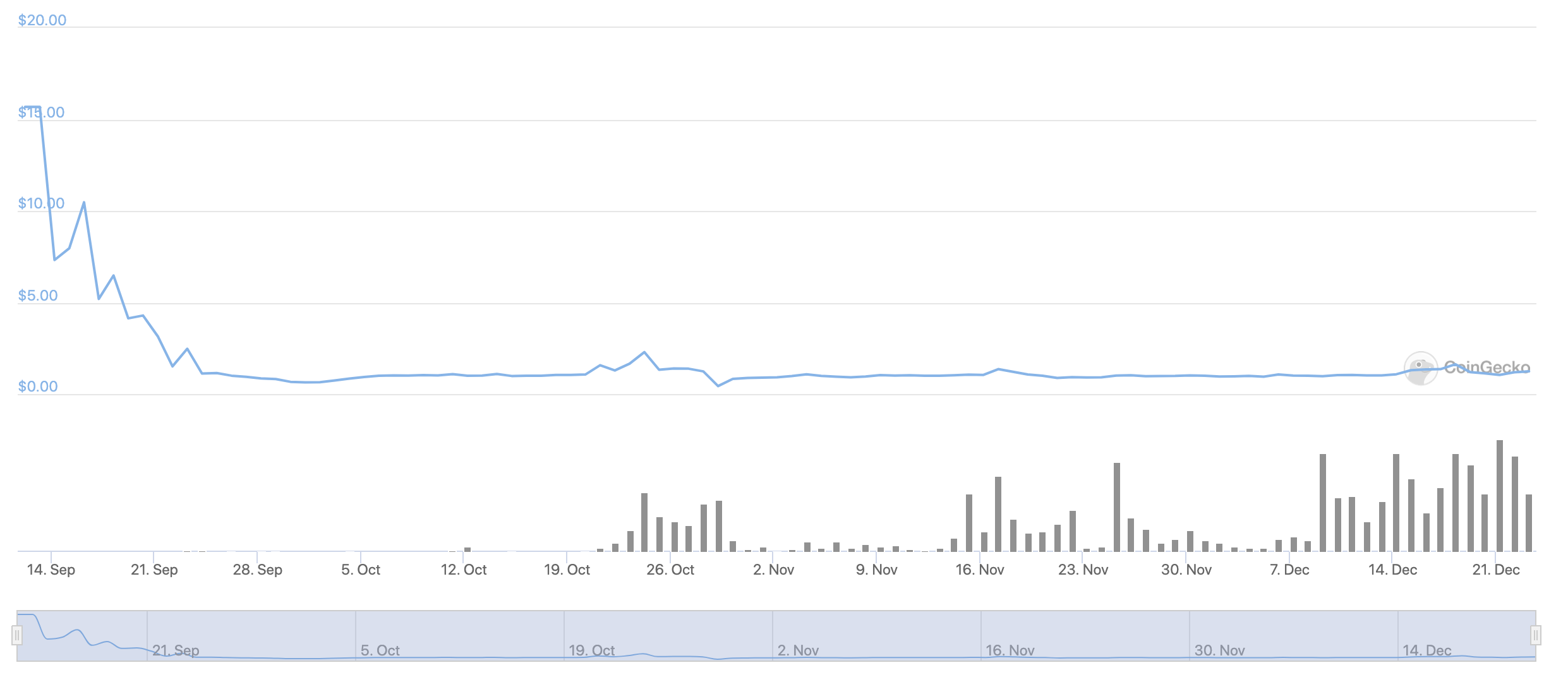
Basis Cash

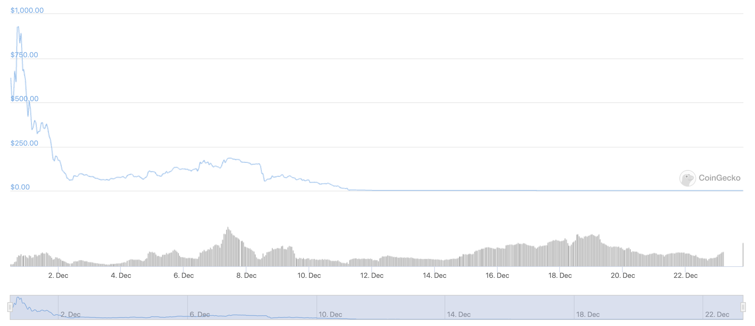
Price Profile (BAC/USD)

Stability starts

Basis Cash

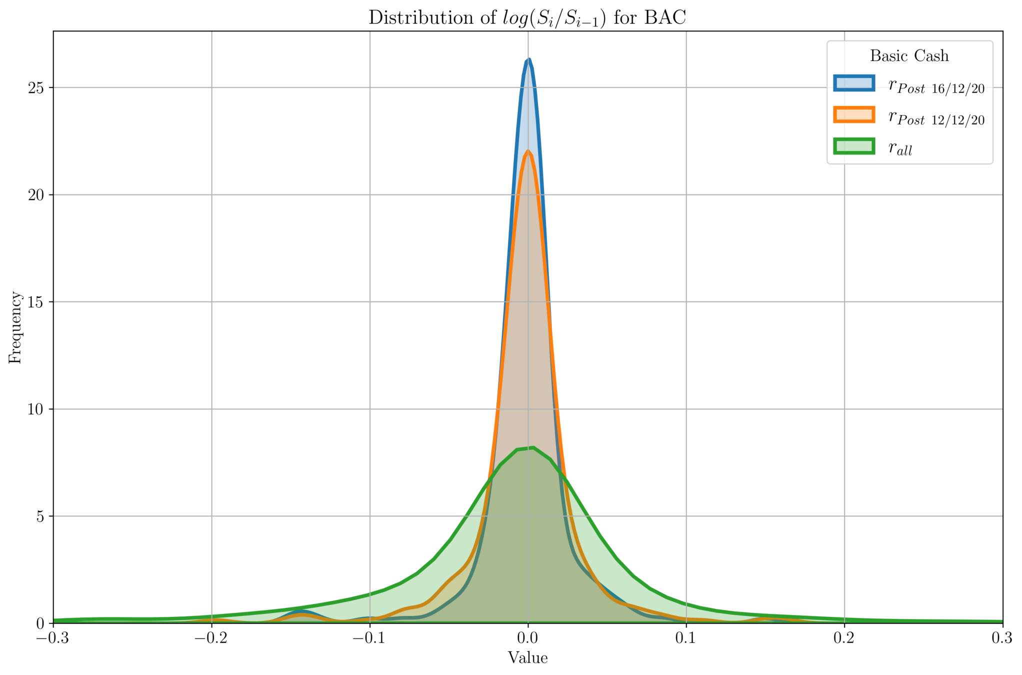
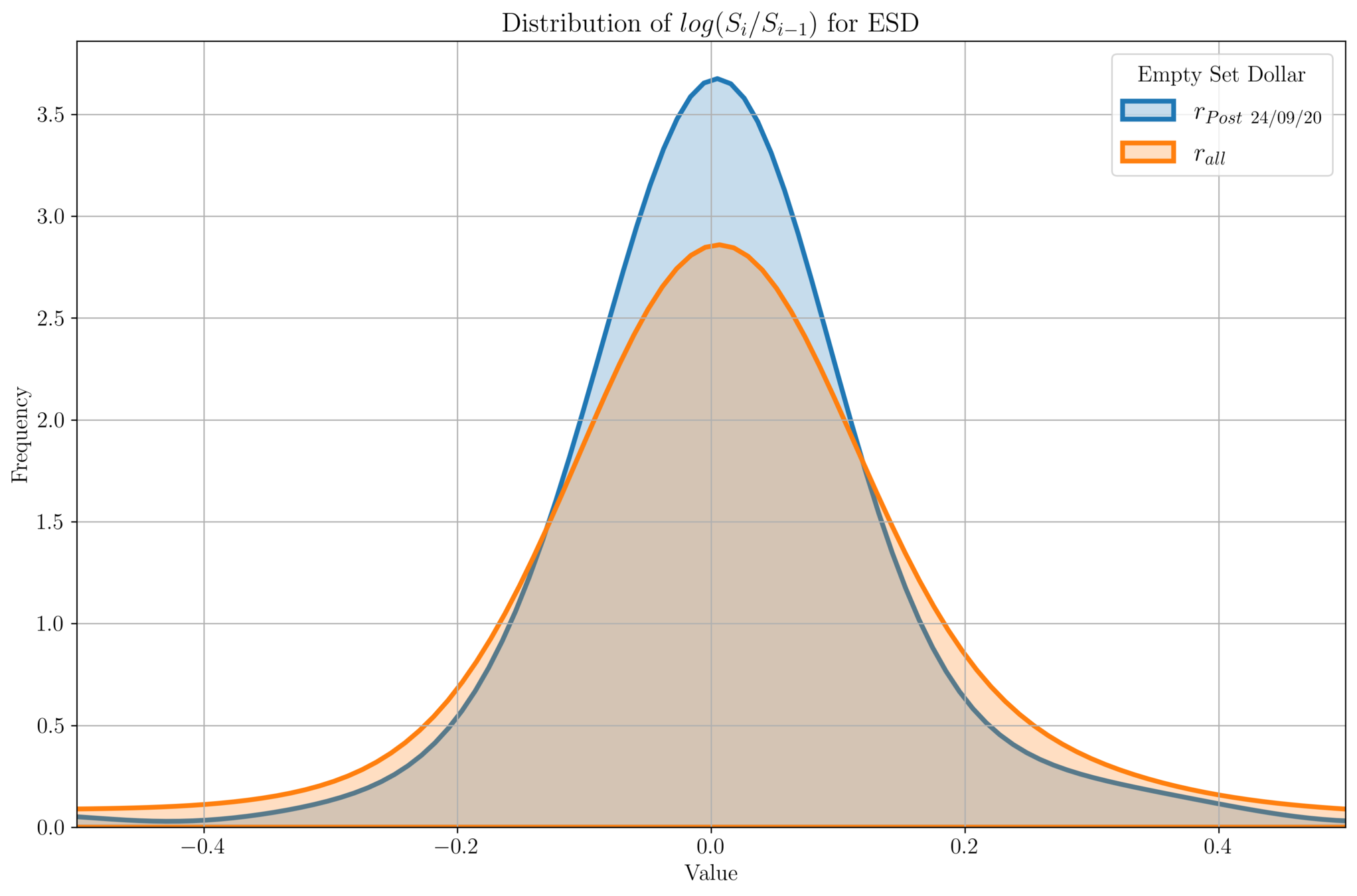
We plot the distribution of $\text{log}\left(\frac{S_i}{S_{i-1}}\right)$ for price data $\{S_i\}$ .
Ideally for stablecoins, we should have a delta function at $X = 0$ .
For all the price data, we see a Gaussian distribution centered at 0.
For all-time price data, we see a spread around $[-0.2, 0.2]$ .
For more recent price data (which is stabilized around $\$1$ , we see the variance gets smaller.

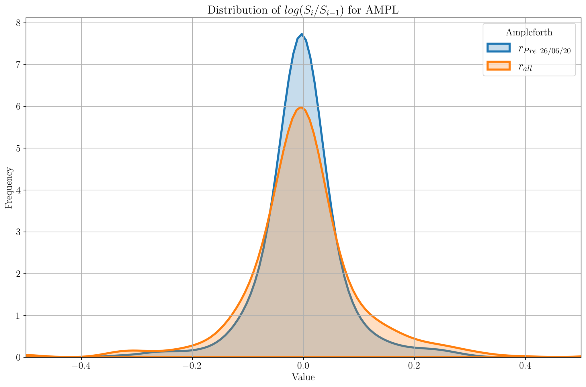
Ampleforth

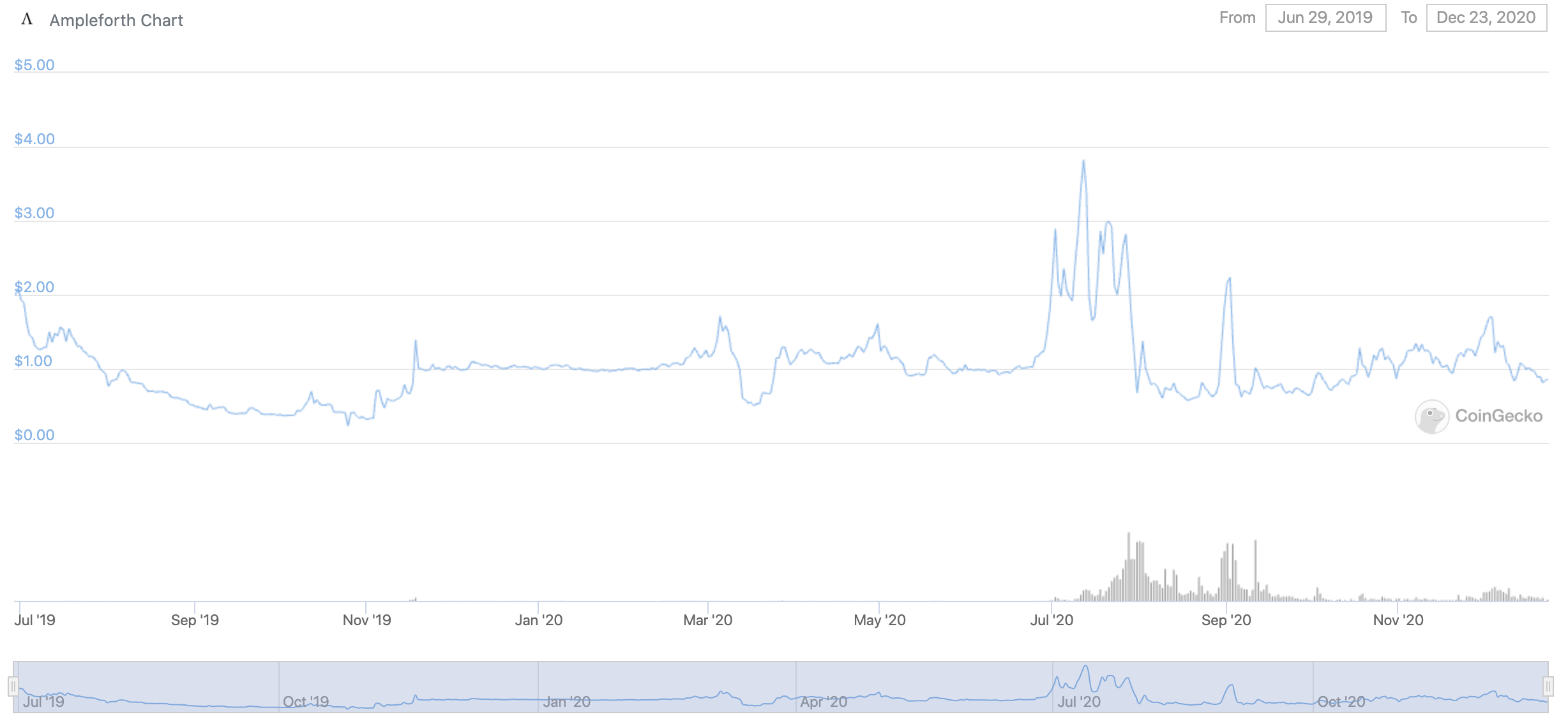
Prices before June 26th are more stable ( $\sim \$1$ ).
Volume trade increase led to price fluctuations.
Here too, we expect the distribution of prices to be Gaussian.

Ampleforth

Empty Set D $\phi$ llar

Drift & Volatility Analysis

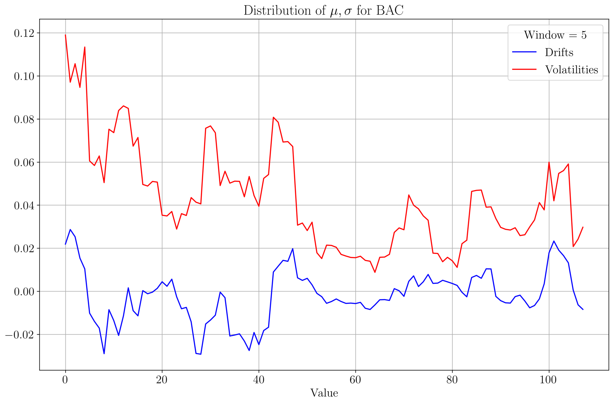
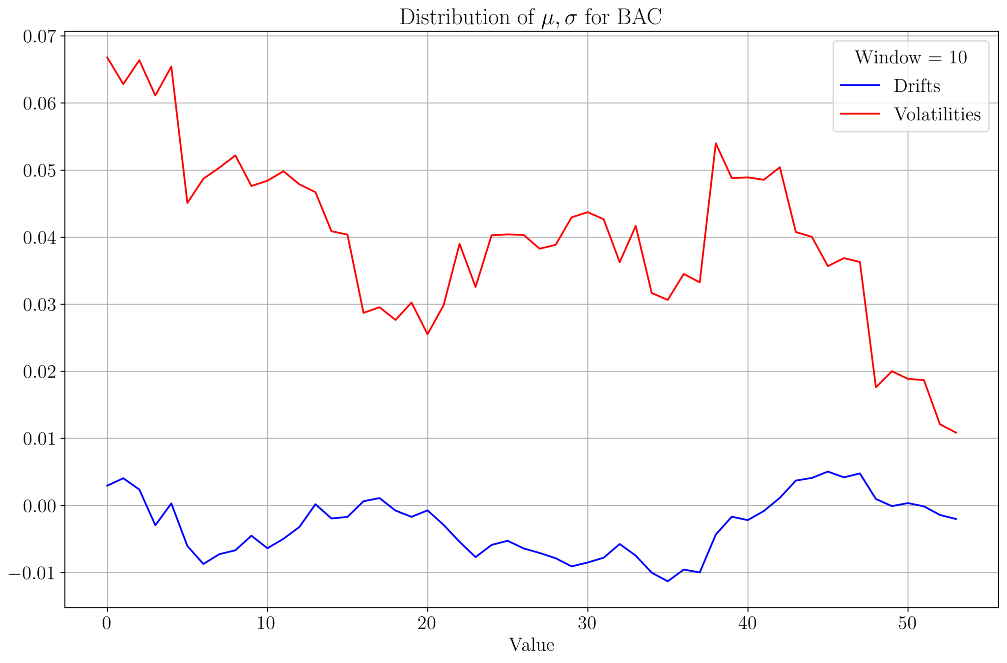
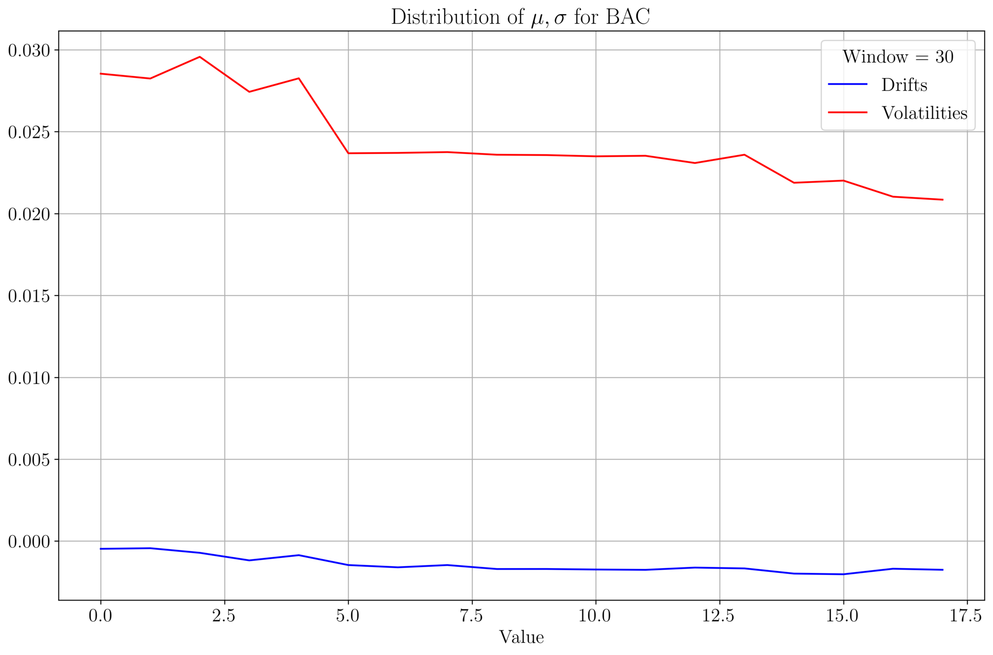
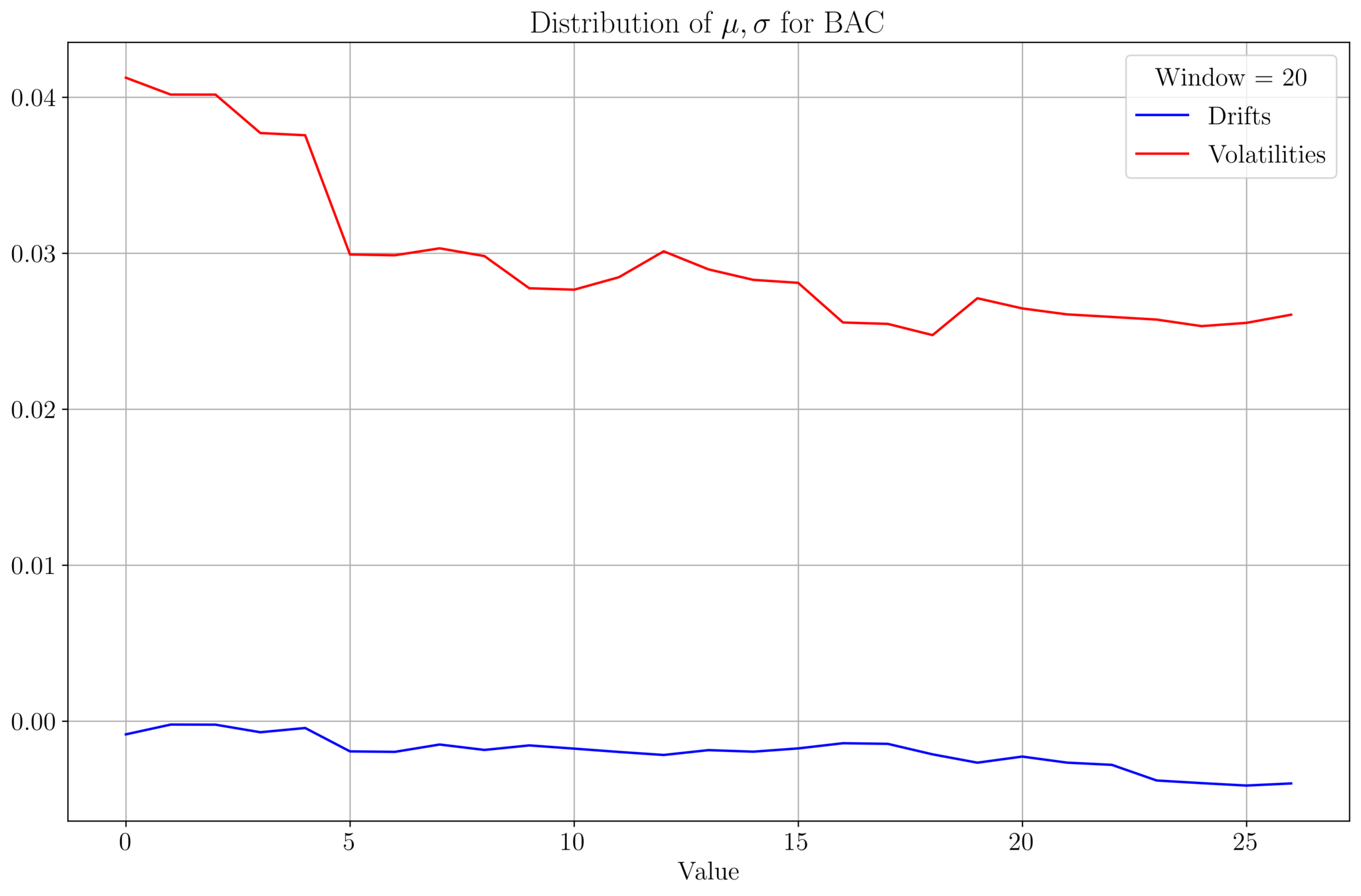
We analyse $\mu, \sigma$ of BAC prices for a data set of size 542.
Plot of $(\mu, \sigma)$ values for a given window size:

Drift & Volatility Analysis

As the window size increases, $\mu, \sigma$ tends to stabilize
$\mu$ and $\sigma$ roughly follow a similar profile

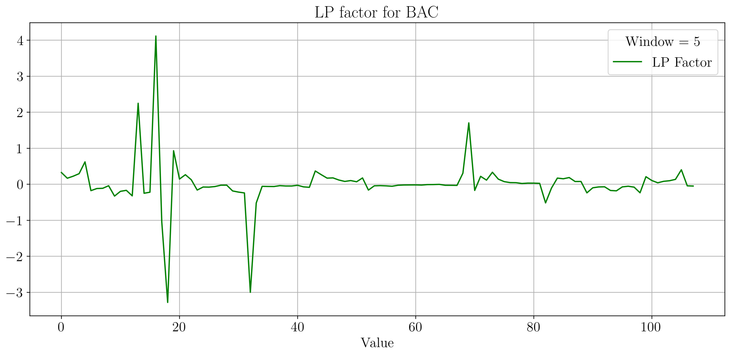
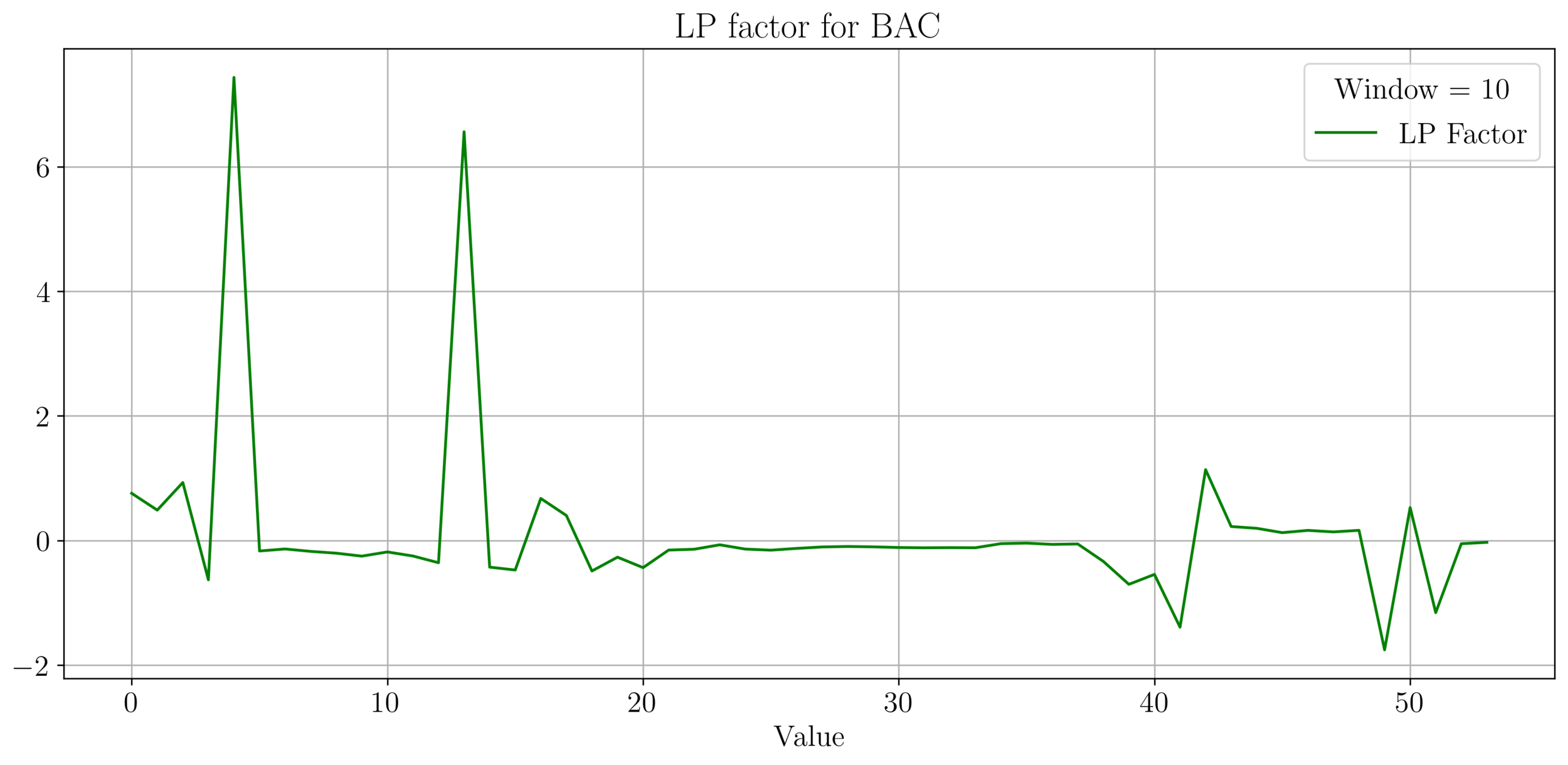
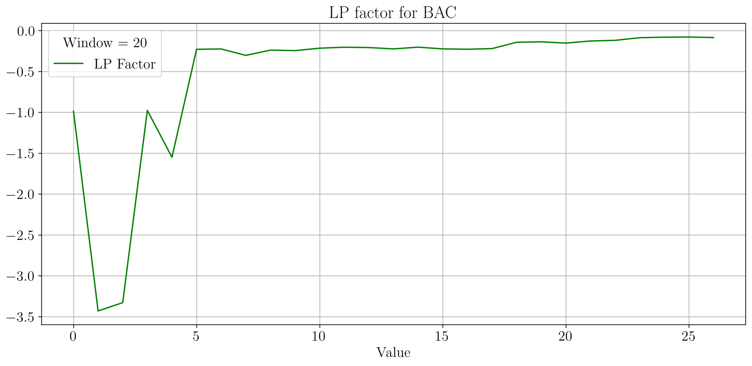
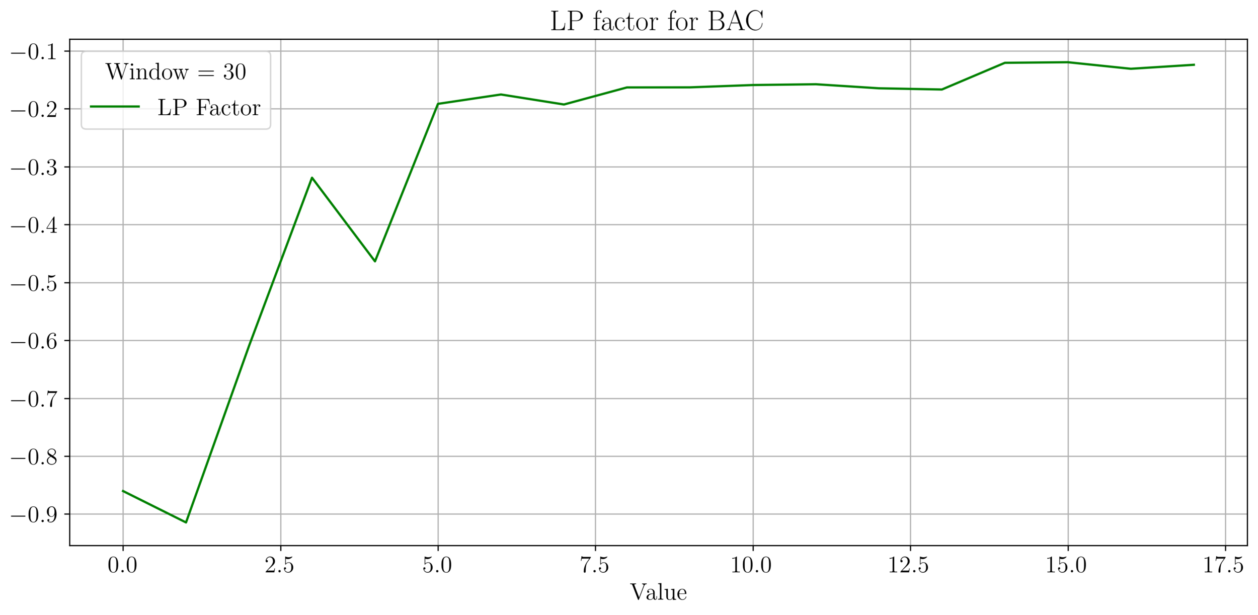
LP Wealth Factor

We plot the factor $f = \frac{\sigma^2}{2\mu}$ , for max LP wealth growth, we want $f \in (0.66, 2)$ .
We observe an irregular pattern here, need more investigation on this.

Price Modelling of Stablecoins