Entropy and information theory
Trang Le, PhD
2021-04-05
Guest lecture
Foundations of AI
@trang1618

Goal: to remain calm under buzzword pressure.
- Entropy
- Microstate
- Macrostate
- Information gain
- Mutual information
- KL divergence
- Epistasis
and some applications...
Quick review: Expected value \(E\)
You toss a fair coin.
- If heads, + $1.
- If tails, \(-\) $1.
What's the expected value of your winning?
Expected winning = \((+\$1)\times 0.5 + (-\$1)\times 0.5= \$0.\)
\[p_{heads}\]
\[p_{tails}\]
Quick review: Expected value \(E\)
\[E[X] = \sum_{i=1}^k x_ip_i = x_1p_1 + x_2p_2 + \cdots + x_kp_k\]
If you play this game \(n\) times, as \(n\) grows, the average will almost surely converge to this expected value.
What if \(p_{heads} = 0.8, p_{tails} = 0.2\) ?
Expected winning = \((+1)\times 0.8 + (-1)\times 0.2 = 0.6.\)
What is entropy?
- disorder?
- uncertainty?
- surprise?
- information?

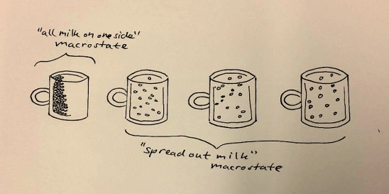
A microstate specifies the position and velocity of all the atoms in the coffee.
A macrostate specifies temperature, pressure on the side of the cup, total energy, volume, etc.
Boltzmann entropy
- themodynamics/statistical mechanics
a
Boltzmann constant
number of configurations
a
\[S = - k_B\sum_i p_i\log p_i = k_B\log \Omega\]
(assume each microstate is equally probable)
\[S = - k_B\sum_i p_i\log p_i\]
expected value of
log(probability that a microstate \(i\) is occupied)
[J/K]
The second law of thermodynamics states that the total entropy of an isolated system can never decrease over time, and is constant if and only if all processes are reversible.
Entropy always increases.
Why is that?
Because it's overwhelmingly more likely that it will.
-- Brian Cox
Shannon entropy
- information theory: expected value of self-information
a
Shannon's entropy
probability of the
possible outcome \(x_i\)
a
\[H(X) = -\sum_{i = 1}^kp(x_i)\log_2p(x_i)\]
[bits]
Source coding theorem.
The Shannon entropy of a model ~ the number of bits of information gain by doing an experiment/sampling on a system your model describes.
An example
\[p_{heads} = 0.5, p_{tails} =0.5\]
\[H = ?\]
\[ H = -p_{heads}log_2(p_{heads})-p_{tails}log_2(p_{tails})\]
\[ = -0.5*log_2(0.5)-0.5*log_2(0.5)\]
\[ = -0.5*(-1)-0.5*(-1) = 1\]
Source coding theorem.
The Shannon entropy of a model ~ the number of bits of information gain by doing an experiment on a system your model describes.
\[H(X) = -\sum_{i = 1}^kp(x_i)\log_2p(x_i)\]
Source coding theorem.
The Shannon entropy of a model ~ the number of bits of information gain by doing an experiment on a system your model describes.
\[p_{heads} = 0.5, p_{tails} =0.5\]
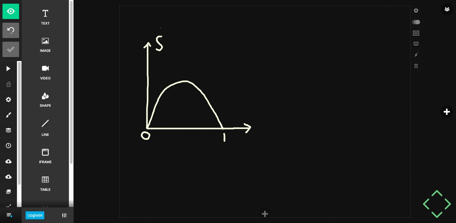
\[H = 1\]
What if \(p_{heads} = 1, p_{tails} =0\)?
\[H = 0\]
What if \(p_{heads} = 0, p_{tails} =1\)?
\[H = 0\]

\[p_{heads}\]

\[H(X) = -\sum_{i = 1}^kp(x_i)\log_2p(x_i)\]
other quantities
Joint entropy
\[H(X|Y) = -\sum_{x \in X, y \in Y}p(x, y)\log_2\frac{p(x, y)}{p(y)}= H(X,Y) - H(Y)\]
Conditional entropy
\[H(X) = -\sum_{x \in X}p(x)\log_2p(x)\]
Entropy
\[H(X, Y) = -\sum_{x \in X}\sum_{y \in Y}p(x, y)\log_2p(x, y)\]
Mutual information
\[I(X;Y)= H(X) - H(X|Y)\]
\[= H(X) + H(Y) - H(X,Y)\]
joint entropy
\[I(X;Y)= D_{KL}(P_{X,Y}|P_X \times P_Y)\]
Kullback-Leibler divergence
a
Discrete probability distributions \(P\) and \(Q\) defined on probability space \(X\)
\[D_{KL}(p|q) = \sum_{x \in X} p(x) \log\frac{p(x)}{q(x)}\]
Cross entropy
\[H_q(p) = \sum_{x\in X} p(x) \log\frac{1}{q(x)}\]
Some applications
of information theory
The gain in phenotype/class information obtained by considering A and B jointly beyond the class information that would be gained by considering variables A and B independently.
\[I(A,B; C) = I(AB;C) - I(A;C) - I(B;C)\]
a
information gained about the phenotype C when locus A is known
information gained about the phenotype C when locus B is known
a
joint attribute constructed from attributes A and B
a
Let's try this!

Node purity
for feature importance (decision trees, random forest, etc.)


Let S be a sample of training examples
- \(p_+\) is the proportion of positive examples in \(S\)
- \(p_-\) is the proportion of negative examples in \(S\)
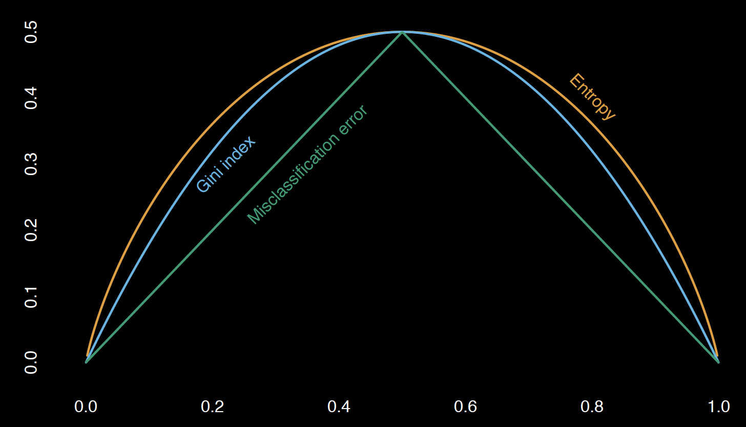
Entropy measures the impurity of \(S\).
\[ Entropy(S) = -p_+log_2(p_+)-p_-log_2(p_-)\]
Information gain = Entropy decrease
\[ Gain(S,model) = Entropy(S) - \sum_{v \in Values(model)} \frac{|S_v|}{|S|}Entropy(S_v)\]
A decision tree example
What is the entropy of \(S\)?
\(S: [9+, 5-]\)
\(p_+ = 9/14, p_- = 5/14\)
\[ Entropy(S) = -p_+log_2(p_+)-p_-log_2(p_-)\]
\[ = -\frac{9}{14}log_2\frac{9}{14}-\frac{5}{14}log_2\frac{5}{14}\]
\[ \approx 0.94\]
+
+
+
+
+
+
+
+
+
+
\(-\)
\(-\)
\(-\)
\(-\)
\(-\)
\(S\)

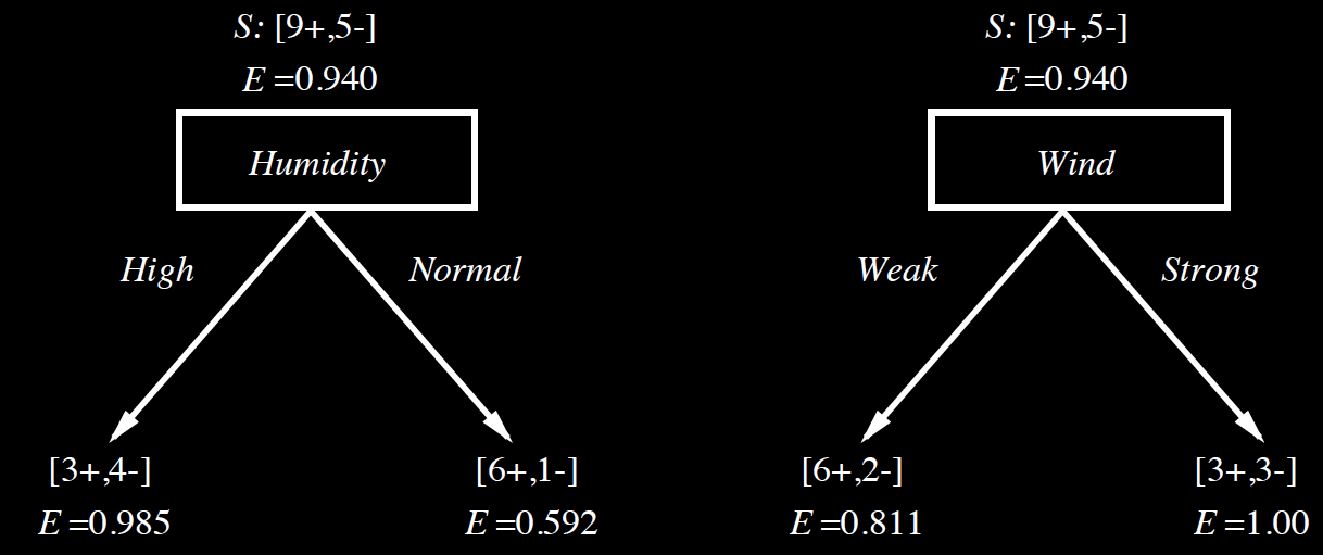
Which one is the better classifier?
\[ Gain(S,model) = Entropy(S) - \sum_{v \in Values(model)} \frac{|S_v|}{|S|}Entropy(S_v)\]
\(Gain(S, Humidity)\)
\(= 0.94-\frac{7}{14}0.985- \frac{7}{14}0.592\)
\(= 0.152\)
\(Gain(S, Wind)\)
\(= 0.94-\frac{8}{14}0.811- \frac{6}{14}(1)\)
\(= 0.048\)
Additional resources
Wikipedia
“Only entropy comes easy.”
-Anton Chekhov