Tidytext chapter 8

NASA datasets' metadata

metadata

32,000 NASA datasets

```
nasa_title
```
```
nasa_desc
```
```
nasa_keyword
```

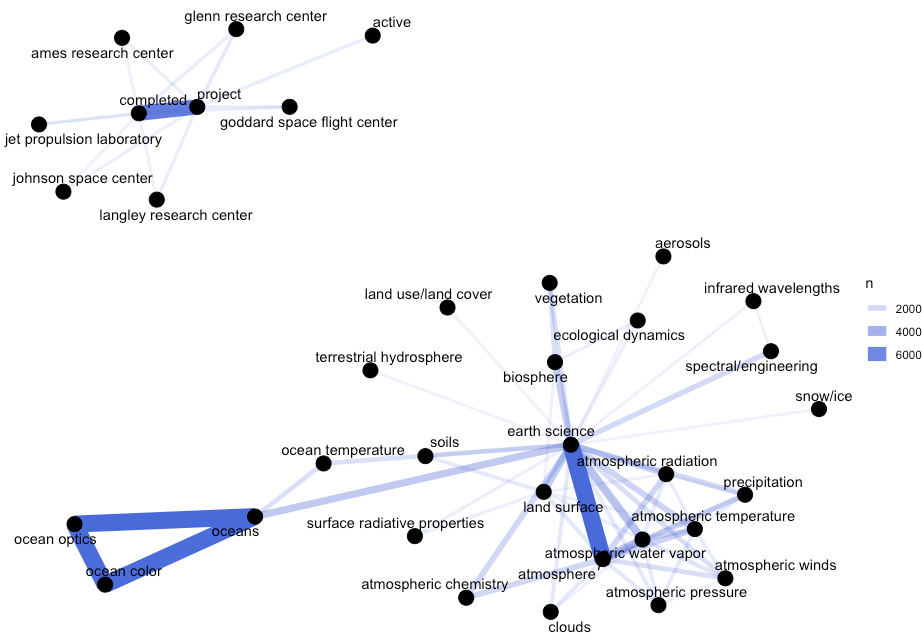
word co-occurrences
word correlations
tf-idf
topic modeling

anti_join(stop_words) to remove stop words
pairwise_count() to count co-occurences of pairs of words

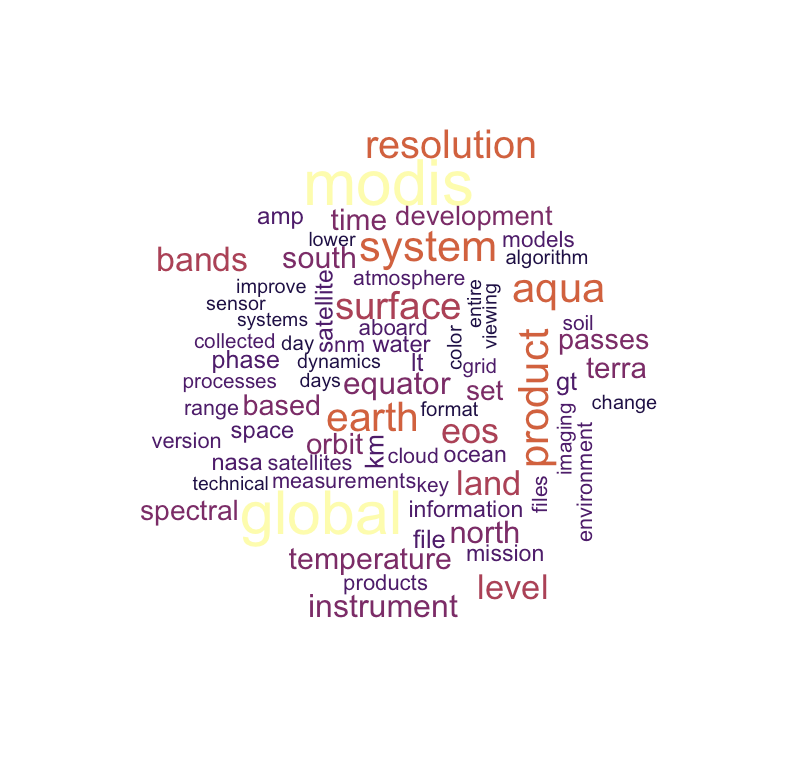
Exercise 1. Create a wordcloud from nasa_desc after removing the word "data"

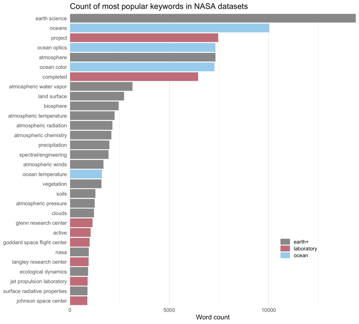
Exercise 2. From nasa_keyword, create a chart of the 30 most popular keywords' counts

*bonus point if colored by `keyword_type`

tf-idf measures how important a word is to a document in a collection of documents

desc_tf_idf <- nasa_desc %>% 
  count(id, word, sort = TRUE) %>%
  ungroup() %>%
  bind_tf_idf(word, id, n)

but...

# A tibble: 1,913,224 x 6
   id                  word                                 n    tf   idf tf_idf
   <chr>               <chr>                            <int> <dbl> <dbl>  <dbl>
 1 55942a7cc63a7fe59b… rdr                                  1     1 10.4   10.4 
 2 55942ac9c63a7fe59b… palsar_radiometric_terrain_corr…     1     1 10.4   10.4 
 3 55942ac9c63a7fe59b… palsar_radiometric_terrain_corr…     1     1 10.4   10.4 
 4 55942a7bc63a7fe59b… lgrs                                 1     1  8.77   8.77
 5 55942a7bc63a7fe59b… lgrs                                 1     1  8.77   8.77

n = 1 and tf = 1 ⇒ description fields that only had a single word in them

desc_tf_idf %>% 
  filter(!near(tf, 1)) %>%
  filter(keyword %in% c("SOLAR ACTIVITY", "CLOUDS", 
                        "SEISMOLOGY", "ASTROPHYSICS",
                        "HUMAN HEALTH", "BUDGET")) %>%
  arrange(desc(tf_idf)) %>%
  group_by(keyword) %>%
  distinct(word, keyword, .keep_all = TRUE) %>%
[...]

Exercise 3. Choose 3 keywords of your choice and plot the words with highest tf-idf for each keyword

topic modeling fits documents into "topics"

# not run
# desc_lda <- LDA(
#   desc_dtm, k = 24, 
#   control = list(seed = 1234)
# )
load("data/desc_lda.rda")

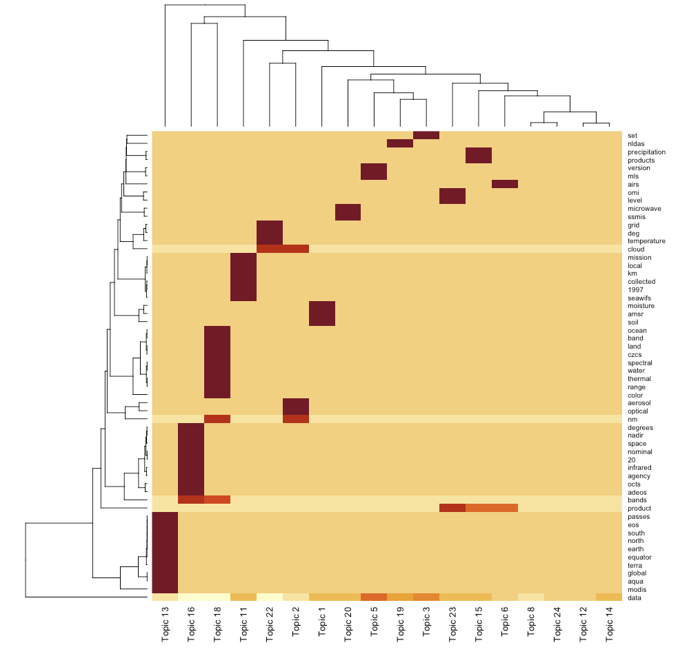
Exercise 4. Create a heatmap of the topic modeling result

> tidy_lda
# A tibble: 861,624 x 3
   topic term       beta
   <int> <chr>     <dbl>
 1     1 suit  1.00e-121
 2     2 suit  2.63e-145
 3     3 suit  1.92e- 79
 4     4 suit  6.72e- 45
 5     5 suit  1.74e- 85
 6     6 suit  7.69e- 84
 7     7 suit  3.28e-  4
 8     8 suit  3.74e- 20
 9     9 suit  4.85e- 15
10    10 suit  4.77e- 10

> beta_mat[1:5, 1:5]
        Topic 16    Topic 1    Topic 2    Topic 3    Topic 5
space 0.02505979 0.00000000 0.00000000 0.00000000 0.00000000
data  0.00000000 0.04488960 0.02154832 0.06751236 0.07210298
nm    0.00000000 0.00000000 0.03450151 0.00000000 0.00000000
soil  0.00000000 0.03676198 0.00000000 0.00000000 0.00000000
level 0.00000000 0.00000000 0.00000000 0.00000000 0.00000000