Topic modeling
Chapter 6, Text Mining with R

Every document is a mixture of topics.
Every topic is a mixture of words.
library(topicmodels)

data("AssociatedPress")
AssociatedPress
#> <<DocumentTermMatrix (documents: 2246, terms: 10473)>>
#> Non-/sparse entries: 302031/23220327
#> Sparsity           : 99%
#> Maximal term length: 18
#> Weighting          : term frequency (tf)
# set a seed so that the output of the model is predictable
ap_lda <- LDA(
AssociatedPress,
k = 2,
control = list(seed = 1234)
)
ap_lda
#> A LDA_VEM topic model with 2 topics.
library(tidytext)

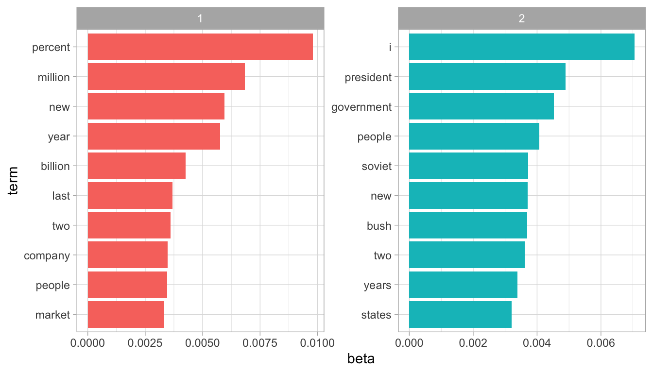
ap_topics <- tidy(ap_lda, matrix = "beta")
ap_topics
#> # A tibble: 20,946 x 3
#>    topic term           beta
#>    <int> <chr>         <dbl>
#>  1     1 aaron      1.69e-12
#>  2     2 aaron      3.90e- 5
#>  3     1 abandon    2.65e- 5
#>  4     2 abandon    3.99e- 5
#>  5     1 abandoned  1.39e- 4
#>  6     2 abandoned  5.88e- 5
#>  7     1 abandoning 2.45e-33
#>  8     2 abandoning 2.34e- 5
#>  9     1 abbott     2.13e- 6
#> 10     2 abbott     2.97e- 5
#> # … with 20,936 more rows
library(tidyr)

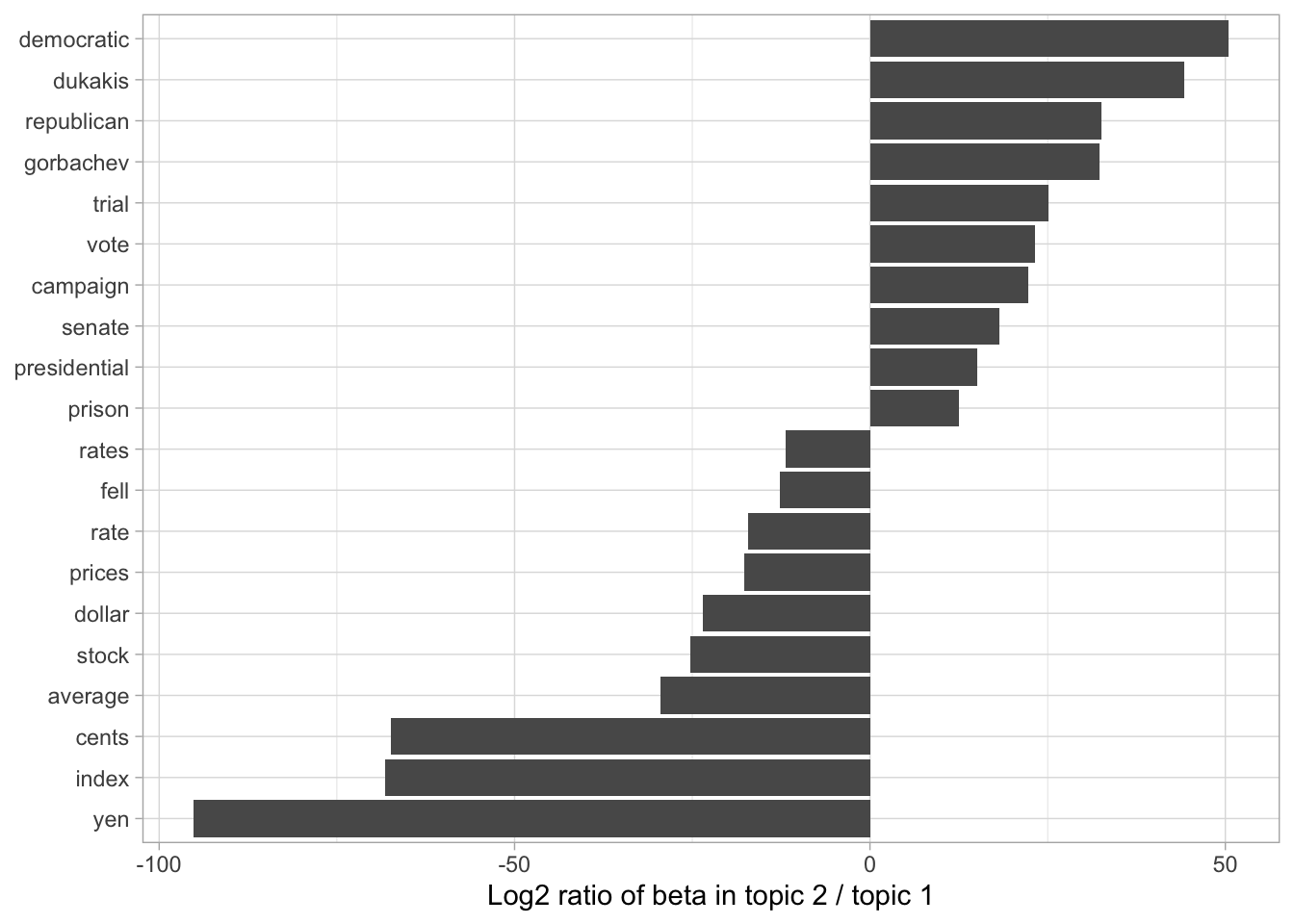
beta_spread <- ap_topics %>%
  mutate(topic = paste0("topic", topic)) %>%
  spread(topic, beta) %>%
  filter(topic1 > .001 | topic2 > .001) %>%
  mutate(log_ratio = log2(topic2 / topic1))

beta_spread
#> # A tibble: 198 x 4
#>    term              topic1      topic2 log_ratio
#>    <chr>              <dbl>       <dbl>     <dbl>
#>  1 administration 0.000431  0.00138         1.68
#>  2 ago            0.00107   0.000842       -0.339
#>  3 agreement      0.000671  0.00104         0.630
#>  4 aid            0.0000476 0.00105         4.46
#>  5 air            0.00214   0.000297       -2.85
#>  6 american       0.00203   0.00168        -0.270
#>  7 analysts       0.00109   0.000000578   -10.9
#>  8 area           0.00137   0.000231       -2.57
#>  9 army           0.000262  0.00105         2.00
#> 10 asked          0.000189  0.00156         3.05
#> # … with 188 more rows

gamma vs. beta
augment
While tidy() retrieves the statistical components of the model, augment() uses a model to add information to each observation in the original data.
Alternative LDA implementations
{mallet}
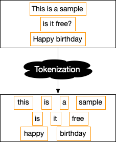
- performs the tokenization itself
- requires a separate file of stopwords
- text needs to be collapsed into one string for each document before performing LDA

My favorite implementation of topic modeling in #rstats is the structural topic model: {stm}
— Julia Silge (@juliasilge) October 10, 2020
🎯Package website: https://t.co/MtYA4XJYP7
🕵️♂️Tutorial for getting started: https://t.co/kG6wvOm6TI
🚀More advanced tutorial (choosing K, etc): https://t.co/WxoeShWWqB pic.twitter.com/0HkEcrtYk0
evaluation
semantic coherence always goes down with more topics