The database
you didn't know you needed


Scott Steinbeck
- Software Developer
- 15+ Year of experience
- Father
- Hardware Tinkerer
Hobbies
- Coding on my free time
- Overcommitting myself
- Automating everything
- IOT Development
- Teaching Coding/Electronics
- Contributing to open source


The Database Fight




Returning
INSERT INTO favourite_color
VALUES ('James', 'Green'),
       ('Peter', 'Blue'),
       ('John', 'Magenta')
RETURNING id, name, color;| id | name | color |
|---|---|---|
| 1 | James | Green |
| 2 | Peter | Blue |
| 3 | John | Magenta |
CREATE TABLE favourite_color(id Serial, name TEXT, color TEXT);Upsert
On duplicate Key Update
INSERT INTO customers (NAME, email)
VALUES('Microsoft','hotline@microsoft.com')
ON CONFLICT ON CONSTRAINT customers_name_key
DO NOTHING;
INSERT INTO customers (name, email)
VALUES('Microsoft','hotline@microsoft.com')
ON CONFLICT (name)
DO
UPDATE SET email = EXCLUDED.email || ';' || customers.email;COPY storm_events FROM '/path/to/csv' DELIMITER ',' CSV HEADER; IMPORTING DATA
Create function get_car_Price(Price_from int, Price_to int)
returns int
language plpgsql  as
$$
Declare Car_count integer;
  Begin
   select count(*)
   into Car_count
   from Car
   where Car_price between Price_from and Price_to;
   return Car_count;
  End;
$$;
Custom Functions
Select get_car_Price(
  26000,
  70000
);

select get_car_Price(
  Price_from => 26000,
    Price_to => 70000
);

select get_car_Price(
  Price_from := 26000,
    Price_to := 70000
); | PL/Java | Java | https://tada.github.io/pljava/ |
| PL/Lua | Lua | https://github.com/pllua/pllua-ng |
| PL/R | R | https://github.com/postgres-plr/plr |
| PL/sh | Unix shell | https://github.com/petere/plsh |
| PL/v8 | JavaScript | https://github.com/plv8/plv8 |
Common Table Expressions
WITH qb_plays AS (
  SELECT DISTINCT ON (POSITION, playid, gameid) POSITION,
  playid, player_id, gameid
  FROM tracking t
  WHERE POSITION = 'QB'
),
total_qb_plays AS (
  SELECT count(*) play_count, player_id
  FROM qb_plays
  GROUP BY player_id
),
qb_games AS (
	SELECT count(DISTINCT gameid) game_count, player_id
    FROM qb_plays
	GROUP BY player_id
),
sacks AS (
  SELECT count(*) sack_count, player_id
  FROM play p
  INNER JOIN qb_plays ON p.gameid = qb_plays.gameid
         AND p.playid = qb_plays.playid
  WHERE p.passresult = 'S'
  GROUP BY player_id
)
SELECT play_count, game_count, sack_count,
   (sack_count/play_count::float)*100 sack_percentage, display_name
FROM total_qb_plays tqp
INNER JOIN qb_games qg ON tqp.player_id = qg.player_id
LEFT JOIN sacks s ON s.player_id = qg.player_id
INNER JOIN player ON tqp.player_id = player.player_id
ORDER BY sack_count DESC NULLS last;
Temporary Tables with names. An easy way to provide clean syntax for querying multiple sets of data.
Data can then be joined together in the final query
WITH RECURSIVE subordinates AS (
    SELECT employee_id, manager_id, full_name
    FROM employees
    WHERE employee_id = 2
  UNION
    SELECT e.employee_id, e.manager_id, e.full_name
    FROM employees e
    INNER JOIN subordinates s ON s.employee_id = e.manager_id
)

SELECT * FROM subordinates;
Recursive CTE
 employee_id | manager_id |  full_name
-------------+------------+-------------
           2 |          1 | Megan Berry
R0.
employee_id | manager_id |    full_name
------------+------------+-----------------
          6 |          2 | Bella Tucker
          7 |          2 | Ryan Metcalfe
          8 |          2 | Max Mills
          9 |          2 | Benjamin Glover
R1.
employee_id | manager_id |    full_name
------------+------------+-----------------
         16 |          7 | Piers Paige
         17 |          7 | Ryan Henderson
         18 |          8 | Frank Tucker
         19 |          8 | Nathan Ferguson
         20 |          8 | Kevin Rampling
R2.
| ...id | full_name | man.._id |
|---|---|---|
| 1 | Michael North | null |
| 2 | Megan Berry | 1 |
| 3 | Sarah Berry | 1 |
| 4 | Zoe Black | 1 |
| 5 | Tim James | 1 |
| 6 | Bella Tucker | 2 |
| 7 | Ryan Metcalfe | 2 |
| 8 | Max Mills | 2 |
| 9 | Benjamin Glover | 2 |
| 11 | Nicola Kelly | 3 |
| 13 | Dominic King | 3 |
| 20 | Kevin Rampling | 8 |
Top Level Employee ID
Working With Dates
select extract(year from current_date)
// 2021-10-20 -> 2021
date_part() and the standard compliant extract(... from ...)
now() (UTC) Timestamp      current_date (UTC) Timestamp
2021-09-20T16:59:30.464Z   2021-09-20T00:00:00.000Z
NOW() and CURRENT_DATE
WHERE occurred_at >= NOW() - interval '12 hour'AGE(created) AS account_age
AGE(ended_at,started_at) time_to_completeWritten Time From now 6 years 1 mon 25 days 02:57:00
select date_trunc('year', current_date) //2021-10-20 -> 2021-01-01date_trunc() "rounds" the value to the specified precision.
Range Types
• Conference schedule
• Budget for buying a new laptop
SELECT *
FROM cars
WHERE
  (
    cars.min_price ≤ 13000 AND
    cars.min_price ≤ 15000 AND
    cars.max_price ≥ 13000 AND
    cars.max_price ≤ 15000
) OR (
    cars.min_price ≤ 13000 AND
    cars.min_price ≤ 15000 AND
    cars.max_price ≥ 13000 AND
    cars.max_price ≥ 15000
) OR (
    cars.min_price ≥ 13000 AND
    cars.min_price ≤ 15000 AND
    cars.max_price ≥ 13000 AND
    cars.max_price ≤ 15000
) OR (
    cars.min_price ≥ 13000 AND
    cars.min_price ≤ 15000 AND
    cars.max_price ≥ 13000 AND
    cars.max_price ≥ 15000
  )
ORDER BY cars.min_price;
SELECT *
FROM cars
WHERE cars.price_range
&< int4range(13000, 15000)
ORDER BY lower(cars.price_range);
id | name | price_range
----+---------------------+---------------
2 | Buick Skylark | [2000,4001)
3 | Pontiac GTO | [5000,7501)
4 | Chevrolet Camaro | [10000,12001)
5 | Ford Mustang | [11000,15001)
6 | Lincoln Continental | [12000,14001)OR
=  equal
<> not equal
<  less than
>  greater than
<= less than
   or equal
>= greater than
   or equal
@> contains range
<@ range is contained by
&& overlap
(have points in common)
<< strictly left of
>> strictly right of
&< not extend to the right of
&> not extend to the left ofMaterialized Views
CREATE MATERIALIZED VIEW sales_summary AS
  SELECT
      seller_no,
      invoice_date,
      sum(invoice_amt)::numeric(13,2) as sales_amt
    FROM invoice
    WHERE invoice_date < CURRENT_DATE
    GROUP BY
      seller_no,
      invoice_date
    ORDER BY
      seller_no,
      invoice_date;

CREATE UNIQUE INDEX sales_summary_seller
  ON sales_summary (seller_no, invoice_date);
Temporary Tables with names. An easy way to provide clean syntax for querying multiple sets of data.
Data can then be joined together in the final query
REFRESH MATERIALIZED VIEW sales_summary;
REFRESH MATERIALIZED VIEW CONCURRENTLY sales_summary;
Faster than a view (stored on disk)
Indexable like a standard table
Easy to refresh data and can be refreshed concurrently with unique index
JSON/JSONB
JSONB Column
jsonb: no whitespaces
jsonb: no duplicate keys, last key wins
jsonb: keys are sorted

SELECT info -> 'customer' AS customer
FROM orders;

SELECT info -> 'items' ->> 'product' as product
FROM orders
ORDER BY product;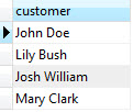

JSON Column
json: textual storage «as is»
JsQuery – json query language with GIN indexing support
Select *
From bookmarks
where json_data @>  '{"tags":[{"term":"NYC"}]}'
-- Find bookmarks with tag NYC
CREATE TABLE mailing_list (
id SERIAL PRIMARY KEY,
first_name VARCHAR NOT NULL,
last_name VARCHAR NOT NULL,
email VARCHAR NOT NULL,
CHECK (
first_name !~ '\s'
AND last_name !~ '\s'
)
);In this table, both first_name and last_name columns
DO NOT ACCEPT null and spaces
row_to_json (table data to JSON)
INSERT INTO employees
 (department_id, name, start_date, fingers, geom)
VALUES
 (1, 'Paul',   '2018/09/02', 10, 'POINT(-123.32977 48.40732)'),
 (1, 'Martin', '2019/09/02',  9, 'POINT(-123.32977 48.40732)'),
 (2, 'Craig',  '2019/11/01', 10, 'POINT(-122.33207 47.60621)'),
 (2, 'Dan',    '2020/10/01',  8, 'POINT(-122.33207 47.60621)');

SELECT row_to_json(employees)
FROM employees
WHERE employee_id = 1;
PostgreSQL has built-in JSON generators that can be used to create structured JSON output right in the database.
{
  "employee_id": 1,
  "department_id": 1,
  "name": "Paul",
  "start_date": "2018-09-02",
  "fingers": 10,
  "geom": {
    "type": "Point",
    "coordinates": [
      -123.329773,
      48.407326
    ]
  }
}
Returns each row serialized to JSON
.... but i want my whole dataset of results to be serialized...
As you wish!

Full result sets using json_agg
INSERT INTO employees
 (department_id, name, start_date, fingers, geom)
VALUES
 (1, 'Paul',   '2018/09/02', 10, 'POINT(-123.32977 48.40732)'),
 (1, 'Martin', '2019/09/02',  9, 'POINT(-123.32977 48.40732)'),
 (2, 'Craig',  '2019/11/01', 10, 'POINT(-122.33207 47.60621)'),
 (2, 'Dan',    '2020/10/01',  8, 'POINT(-122.33207 47.60621)');

SELECT json_agg(e)
FROM (
    SELECT employee_id, name
    FROM employees
    WHERE department_id = 1
) e;
[
{
"employee_id": 1,
"name": "Paul"
},
{
"employee_id": 2,
"name": "Martin"
}
]json_agg converts the multiple results into a JSON list.
.... but I was to see all of the employees grouped by department...

json_agg contined...
WITH
-- strip down employees table
employees AS (
  SELECT department_id, name, start_date
  FROM employees
),
-- join to departments table and aggregate
departments AS (
  SELECT d.name AS department_name,
         json_agg(e) AS employees
  FROM departments d
  JOIN employees e
  USING (department_id)
  GROUP BY d.name
)
-- output as one json list
SELECT json_agg(departments)
FROM departments;
[
{
"department_name": "cloud",
"employees": [
{
"department_id": 2,
"name": "Craig",
"start_date": "2019-11-01"
},
{
"department_id": 2,
"name": "Dan",
"start_date": "2020-10-01"
}
]
},
{
"department_name": "spatial",
"employees": [
{
"department_id": 1,
"name": "Paul",
"start_date": "2018-09-02"
}...Let's use a Common Table Expression to serialize the employees and then we can join them to departments
Export table schema as JSON
WITH rows AS (
  SELECT c.relname, a.attname, a.attnotnull, a.attnum, t.typname
  FROM pg_class c
  JOIN pg_attribute a
    ON c.oid = a.attrelid and a.attnum >= 0
  JOIN pg_type t
    ON t.oid = a.atttypid
  JOIN pg_namespace n
    ON c.relnamespace = n.oid
  WHERE n.nspname = 'public'
    AND c.relkind = 'r'
),
agg AS (
  SELECT rows.relname, json_agg(rows ORDER BY attnum) AS attrs
  FROM rows
  GROUP BY rows.relname
)

-- finally we use json_object_agg to assign the json rows as to a key
SELECT json_object_agg(agg.relname, agg.attrs)
FROM agg;
{
"departments": [
{
"relname": "departments",
"attname": "department_id",
"attnotnull": true,
"attnum": 1,
"typname": "int8"
},
{
"relname": "departments",
"attname": "name",
"attnotnull": false,
"attnum": 2,
"typname": "text"
}
],
...
}This will use the PostgreSQL system tables to grab and group tables and columns into a full JSON db schema
wait is that an order by in the json_agg function?
Aggregate functions
Aggregate functions that support Partial Mode are eligible to participate in various optimizations, such as parallel aggregation
/* A * by the name means it supports partial mode */

/* General-Purpose Aggregate Functions */
 avg*, bit_and*, bit_or*, bool_and*, bool_or*, count*, max*, min*, sum*,
 array_agg, json_agg, json_object_agg,string_agg, xmlagg

/* Aggregate Functions for Statistics */
 corr* (correlation coefficient)
 covar_pop* (population covariance)
 stddev_samp* (standard deviation)
 regr_slope* (slope of the least-squares-fit)
 regr_count* (number of rows in which both inputs are non-null)
 ...

/* Ordered-Set Aggregate Functions */
 mode* (mode of a number set)
 percentile_cont (continuous percentile)
 percentile_disc (discrete percentile)

/* Hypothetical-Set Aggregate Functions */
 rank (rank ordered items with gaps) 1, 1, 3, 4, 4, 6
 dense_rank (rank ordered items with NO gaps) 1, 1, 2, 3, 3, 3, 4
 percent_rank (rank ordered items with % 0-1)
 cume_dist (for calculating the probability of a value randomly being picked)
What might rank be used for?
Window Functions

SELECT COUNT(*) OVER (PARTITION BY MONTH(date_started),YEAR(date_started))
As NumPerMonth,
DATENAME(month,date_started)+' '+DATENAME(year,date_started) As TheMonth,
firstname, lastname
FROM Employee
ORDER BY date_started;| NumPerMonth | TheMonth | Firstname | Lastname |
|---|---|---|---|
| 1 | January 2019 | John | Smith |
| 2 | February 2019 | Sally | Jones |
| 2 | February 2019 | Sam | Gordon |
Window Functions - Row number & Rank
SELECT
  ROW_NUMBER() OVER (ORDER BY YEAR(date_started),MONTH(date_started)) As StartingRank,

  RANK() OVER (ORDER BY YEAR(date_started),MONTH(date_started)) As EmployeeRank,

  DENSE_RANK() OVER (ORDER BY YEAR(date_started),MONTH(date_started)) As DenseRank,

  DATENAME(month,date_started)+' '+DATENAME(year,date_started) As TheMonth,
  firstname, lastname, date_started
FROM Employee
ORDER BY date_started;| StartingRank | EmployeeRank | DenseRank | TheMonth | firstname | lastname | date_started |
|---|---|---|---|---|---|---|
| 1 | 1 | 1 | January 2019 | John | Smith | 2019-01-01 |
| 2 | 2 | 2 | February 2019 | Sally | Jones | 2019-02-15 |
| 3 | 2 | 2 | February 2019 | Sam | Gordon | 2019-02-18 |
| 4 | 4 | 3 | March 2019 | Julie | Sanchez | 2019-03-19 |
Window Functions - Preceding & Following
SELECT OrderYear, OrderMonth, TotalDue,

    SUM(TotalDue) OVER(ORDER BY OrderYear, OrderMonth
                    ROWS BETWEEN UNBOUNDED PRECEDING AND 1 PRECEDING
                  ) AS 'LaggingRunningTotal'
FROM sales_products;
In this example, the window frame goes from:
the first_row to the current_row - 1,
and the window size continues to increase for each row.
Most standard aggregate functions work with Window functions. We’ve seen COUNT in the examples already. Others include SUM, AVG, MIN, MAX, etc.
With window functions, you can also access both previous records and subsequent records using LAG and LEAD, and FIRST_VALUE and LAST_VALUE.
Built-in Search

batteries included
like, regex, & simliarity
1. Prefix + fuzzy query. For this type, B-tree indexes can be used.
select * from tbl where col like 'ab%'; /* or */ select * from tbl where col ~ '^ab';2. Suffix + fuzzy query. ( ~ is for regex expressions )
select * from tbl where col like '%ab';
select * from tbl where col ~ 'ab$';
select * from tbl where reverse(col) like 'ba%';
select * from tbl where reverse(col) ~ '^ba';
<cfcollection> <cfsearch>
3. Full Regexp query. both pg_trgm and GIN indexes can be used.
select * from tbl where col ~ '^a[0-9]{1,5}\ +digoal$';select * from tbl order by similarity(col, 'postgre') desc limit 10;3. Similarity query. both pg_trgm and GIN indexes can be used.
CREATE EXTENSION pg_trgm;Whats a trigram ? 'word' => {" w"," wo","ord","wor","rd "}
Fuzzy Search Using Trigrams
SELECT * FROM storm_events WHERE event_type % 'Drot' -- Similarity
Similarity Search (Score 0-1)
A trigram is a group of three consecutive characters taken from a string.
We can measure the similarity of two strings by counting the number of trigrams they share.
Relax it gets better

Built-in Search
ts_vector, ts_rank, to_tsquery
SELECT  userID, userName, email, username, phone
FROM (
    SELECT
        users.email,
        users.username,
        MEMBER.phone,
        (
          setweight(to_tsvector('simple', coalesce(member.member_number,'') ),'A') ||
          setweight(to_tsvector('simple', coalesce(member.member_number,'') ),'A') ||
          setweight(to_tsvector('simple', coalesce(member.business_name,'') ),'B') ||
          setweight(to_tsvector('simple', coalesce(member.last_name,''    ) ),'B') ||
          setweight(to_tsvector('simple', coalesce(member.first_name,''   ) ),'B') ||
          setweight(to_tsvector('simple', coalesce(member.phone,''        ) ),'C') ||
          setweight(to_tsvector('simple', coalesce(member.address,''      ) ),'D')
        ) as document
    FROM member
    INNER JOIN users ON member.user_id = users.oid
) p_search

WHERE p_search.document @@ to_tsquery('simple', 'tom:*')

ORDER BY ts_rank(p_search.document, to_tsquery('simple', 'tom:*')) DESC
Convert to TS search
calculate rank from query in %
SELECT to_tsquery('english', 'The & Fat & Rats'); -> 'fat' & 'rat'SELECT DISTINCT(event_type) FROM storm_events WHERE DIFFERENCE(event_type, 'he') > 2
SELECT * FROM storm_events WHERE levenshtein(event_type, 'Drot') < 4
Levenshtein Search >= 0
CREATE EXTENSION fuzzystrmatch; the minimum number of single-character edits required for
both the strings/words to match.
Phonetic Match
This will give us all events sounding like 'he'
eg. Heat, Hail
Fuzzy String match
Generate Series
SELECT time, device_id
FROM generate_series(
    '2021-01-01 00:00:00',
    '2021-01-01 11:00:00',
    INTERVAL '1 hour'
  ) as time,
generate_series(1,4)
    as device_id;

time               |device_id|
-------------------+---------+
2021-01-01 00:00:00|        1|
2021-01-01 01:00:00|        1|
2021-01-01 02:00:00|        1|
2021-01-01 03:00:00|        1|
...
SELECT *
from
generate_series(0,12,2);
-- (start, end, step)
generate_series
-----------------
0
2
4
6
8
10
12SELECT *
from
generate_series(1,3) a,
generate_series(4,5) b;
-- (start, end, step)
a |b|
--+-+
1|4|
2|4|
3|4|
1|5|
2|5|
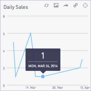
3|5|select date(d) as day,
count(sales.id)
from generate_series(
current_date - interval '30 day',
current_date,
'1 day'
) d
left join sales
on date(sales.created_at) = d
group by day
order by day;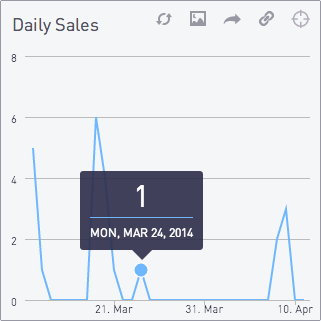
Lateral Joins

Kickstarter Stats
We want to calculate:
- total pledged in USD
- average pledge in USD
select
    pledged_usd,
    avg_pledge_usd,
    amt_from_goal,
    duration,
    (usd_from_goal / duration) as usd_needed_daily
from kickstarter_data,
    lateral (select pledged / fx_rate as pledged_usd) pu
    lateral (select pledged_usd / backers_count as avg_pledge_usd) apu
    lateral (select goal / fx_rate as goal_usd) gu
    lateral (select goal_usd - pledged_usd as usd_from_goal) ufg
lateral (select (deadline - launched_at)/86400.00 as duration) dr;- USD over or under goal
- duration of the project in days
- daily shortfall / surplus, the extra USD needed daily to hit goal
The lateral keyword allows us to access columns after the FROM statement, and reference these columns "earlier" in the query ("earlier" meaning "written higher in the query").
Lateral Joins -
Subselect
The situation is we have a list of orders from customers.
We need to get the top 2 orders for each customer.
| id | user_id | created_at |
|---|---|---|
| 1 | 1 | 2017-06-20 04:35:03 |
| 2 | 2 | 2017-06-20 04:35:07 |
| 3 | 3 | 2017-06-20 04:35:10 |
| 4 | 1 | 2017-06-20 04:58:10 |
| 5 | 3 | 2017-06-20 04:58:17 |
| 6 | 3 | 2017-06-20 04:58:25 |
SELECT user_id, first_order_time, next_order_time, id
FROM (
    SELECT user_id, min(created_at) AS first_order_time
    FROM orders
    GROUP BY user_id
) o1
LEFT JOIN LATERAL (
    SELECT id, created_at AS next_order_time
    FROM orders
    WHERE user_id = o1.user_id AND created_at > o1.first_order_time
    ORDER BY created_at ASC
    LIMIT 1
) o2 ON true;| user_id | first_order_time | next_order_time | id |
|---|---|---|---|
| 1 | 2017-06-20 04:35:03 | 2017-06-20 04:58:10 | 4 |
| 3 | 2017-06-20 04:35:10 | 2017-06-20 04:58:17 | 5 |
Use derived table
Group By or Order By Column Position
Matt Clemente
SELECT
  extract(year FROM b.completed_at) AS yyyy,
  g.name,
  count(b.book_id) AS the_count
FROM
  book AS b
  INNER JOIN genre AS g
          ON b.genre_id = g.genre_id
GROUP BY
  yyyy, g.name
ORDER BY
  yyyy DESC, g.name
SELECT
  extract(year FROM b.completed_at) AS yyyy,
  g.name,
  count(b.book_id) AS the_count
FROM book AS b
INNER JOIN genre AS g
        ON b.genre_id = g.genre_id
GROUP BY
  1, 2
ORDER BY
  1 DESC, 2
Great for aggregate or computed columns
It can be useful but has the downside of returning incorrect data if the select statement changes.
GROUPING SETS: ROLLUP & CUBE
SELECT  country, product_name,
        sum(amount_sold)
FROM    t_sales
GROUP BY GROUPING SETS ((1), (2))
ORDER BY 1, 2;
We have a table with data of hats and shoes sold in many different countries
 country   | product_name | sum
-----------+--------------+-----
 Argentina |              | 137
 Germany   |              | 104
 USA       |              | 373
           | Hats         | 323
           | Shoes        | 291
(5 rows)
Result
SELECT country, product_name,
       sum(amount_sold)
FROM   t_sales
GROUP BY ROLLUP (1, 2)
ORDER BY 1, 2;
country | product | sum
-----------+----------+-----
Argentina | Hats | 111
Argentina | Shoes | 26
Argentina | | 137
Germany | Hats | 41
Germany | Shoes | 63
Germany | | 104
USA | Hats | 171
USA | Shoes | 202
USA | | 373
| | 614
(10 rows)Result
SELECT country, product_name,
       sum(amount_sold)
FROM   t_sales
GROUP BY CUBE (1, 2)
ORDER BY 1, 2;
country | product | sum
-----------+---------+-----
Argentina | Hats | 111
Argentina | Shoes | 26
Argentina | | 137
Germany | Hats | 41
Germany | Shoes | 63
Germany | | 104
USA | Hats | 171
USA | Shoes | 202
USA | | 373
| Hats | 323
| Shoes | 291
| | 614
(12 rows)Result
GROUPING SETS
ROLLUP
CUBE
explain.dalibo.com

Visualizing and understanding PostgreSQL EXPLAIN plans made easy.
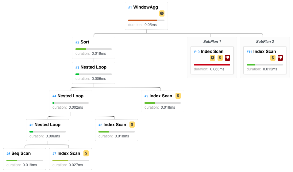
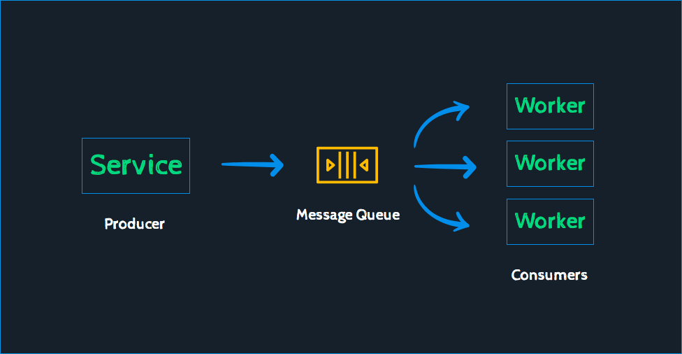
EXPLAIN (ANALYZE, COSTS, VERBOSE, BUFFERS, FORMAT JSON)Message
Queueing
BEGIN; -- start transaction
DELETE FROM
    queue_table
USING (
    SELECT *
    FROM queue_table
    LIMIT 10
    FOR UPDATE
    SKIP LOCKED
) q
WHERE q.id = queue_table.id
RETURNING queue_table.*;
-- return table in using
Requirements:
Must be able to use parallel processing
Auto delete queue items once finished
Don't double process records
Fast SQL operations
pg_timetable: Advanced scheduling for PostgreSQL
Run public.my_func() at 00:05 every day in August Postgres server time zone:
SELECT timetable.add_job(
    'execute-func',
    '5 0 * 8 *',
    'SELECT public.my_func()'
);
Run VACUUM at minute 23 past every 2nd hour from 0 through 20 every day Postgres server time zone:
SELECT timetable.add_job(
    'run-vacuum',
    '23 0-20/2 * * *',
    'VACUUM'
);
Refresh materialized view every 2 hours:
SELECT timetable.add_job(
    'refresh-matview',
    '@every 2 hours',
    'REFRESH MATERIALIZED VIEW
               public.mat_view'
);
Clear log table after pg_timetable restart:
SELECT timetable.add_job(
    'clear-log',
    '@reboot',
    'TRUNCATE timetable.log'
);
-
Tasks can be arranged in chains
-
A chain can consist of built-int commands, SQL and executables
-
Parameters can be passed to chains
-
Support for configurable repetitions
-
Built-in tasks such as sending emails, etc.
Cloud Providers
AWS
GCP
Digital Ocean
Azure
Top Extentions
-
PostGIS
-
Timescale DB
-
PG Backrest
-
Posgres FDW
-
Foreign Data Wrapper
-
GUI
PG Admin
DBeaver
Datagrip
IntelliJ
Navicat (not free)