Compressed Sensing
План
- Постановка проблемы
- L1-регуляризация и некогерентная sensing-матрица
- Теорема 1 (обход Найквиста-Шэннона для разреженного сигнала)
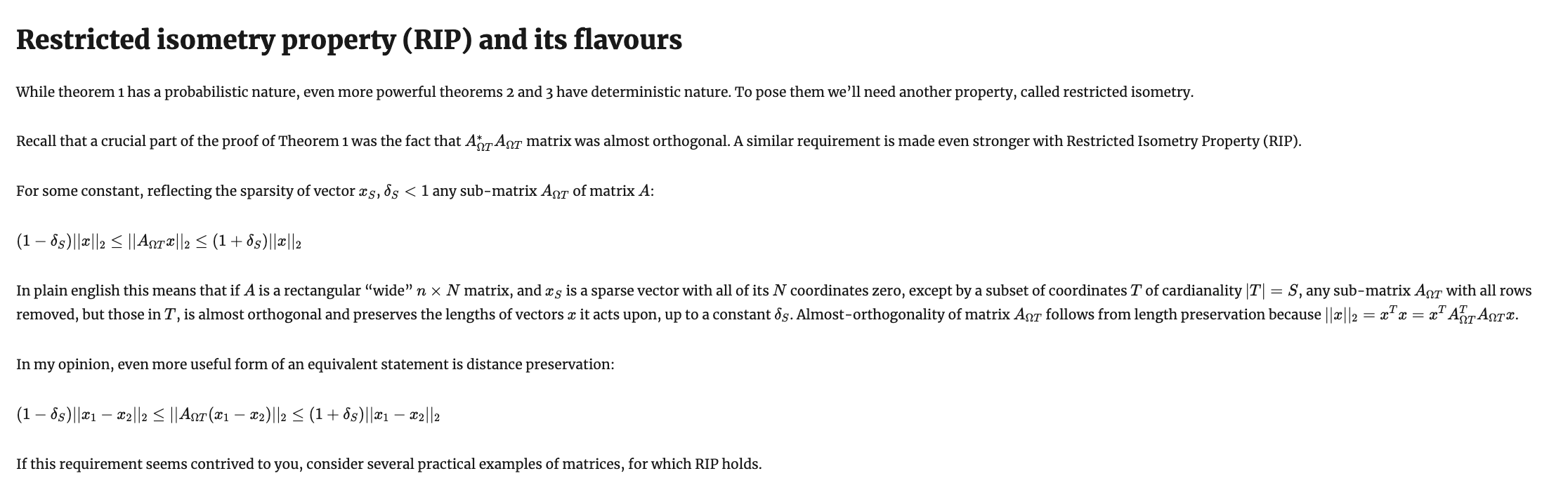
- Restricted Isometry Property и Линденштраусс-Джонсон
- Теорема 2 (если истинный сигнал не разреженный, а почти разреженный - тоже ок)
- Теорема 3 (шум измерений не страшен)
- Обобщения: trace norm'а и низкоранговая аппроксимация вместо разреженности
- Обобщения: разреженные автокодировщики и dictionary learning
Постановка проблемы
Постановка проблемы
Разреженный сигнал
\( A = \Phi \cdot \Psi \) is an \( n \times S \) sensing matrix
\( \Phi \cdot f(t) = \Phi \cdot \Psi \cdot x \), where \( \Phi \) is measurement matrix
\( \Psi \) is sparsifying matrix
Постановка проблемы
Разреженный сигнал
Постановка проблемы
Разреженный сигнал
Постановка проблемы
Разреженный сигнал
Пример разреженного сигнала
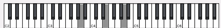
A-E-A chord
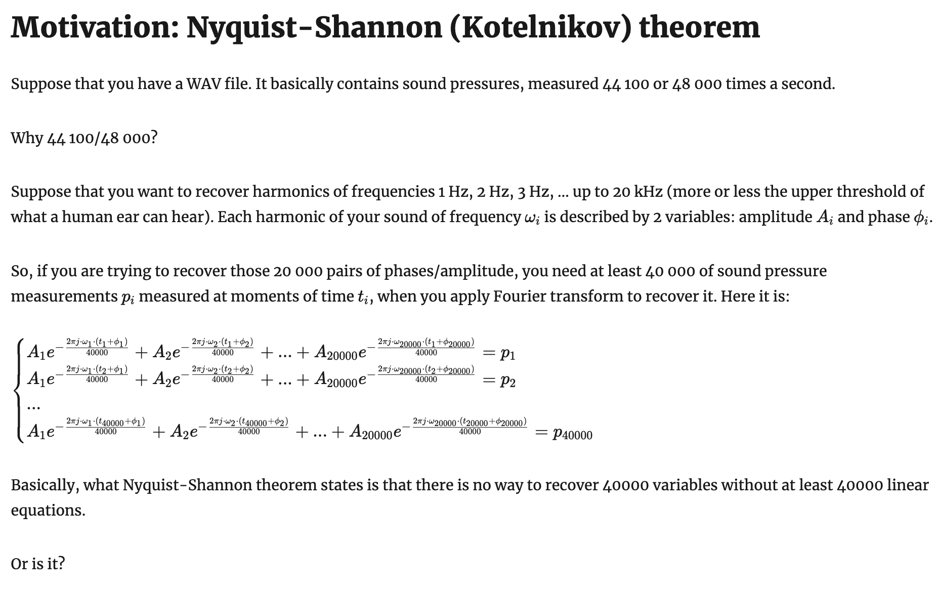
\( f(t) \) - звуковые давления в момент времени t
\( x_i \) - амплитуда i-й гармоники
\( \psi_i(t) \) - i-ая гармоника Фурье или DCT
\( \Phi \) - например, spike-базис дельта-функций
Практический пример
import numpy as np
import matplotlib.pyplot as plt
from scipy import fftpack
from scipy.io import wavfile
from IPython.display import Audio

dim = 48000

a_e_a_chord_dct = np.zeros(dim)

a_e_a_chord_dct[440] = 1
a_e_a_chord_dct[660] = 1
a_e_a_chord_dct[880] = 1


generated_wav = idct(a_e_a_chord_dct)

Audio(generated_wav, rate=dim)
Практический пример
import random
import math

from sklearn import linear_model


# generate a DCT matrix to select just a few random rows from it and use them as a sensing matrix
I = np.identity(dim)
dct_matrix = dct(I)

n_measurements = 100  # measure the sound pressure at this amount of points


def get_random_indices(n_indices=n_measurements, dim=dim):
    output = []
    counter = 0
    while counter < n_indices:
        prospective_random_index = math.floor(random.random() * dim)
        if prospective_random_index not in output:
            output.append(prospective_random_index)
            counter += 1
        else:
            pass  # redraw, if random index was already used

    return output


# select a few rows from our DCT matrix to use this partial DCT matrix as sensing matrix
random_indices = get_random_indices()
partial_dct = np.take(dct_matrix, get_random_indices(), axis=1)

# measure sound pressures at a small number of points by applying sensing matrix to the signal spectrum
y = np.dot(partial_dct.T, a_e_a_chord_dct)

# make the measurement noisy
noise = 0.01 * np.random.normal(0, 1, n_measurements)
signal = y + noise

# recover the initial spectrum from the measurements with L1-regularized regression (implemented as sklearn's Lasso in this case)
lasso = linear_model.Lasso(alpha=0.1)
lasso.fit(partial_dct.T, signal)
for index, i in enumerate(lasso.coef_):
    if i > 0:
        print(f"index = {index}, coefficient = {i}")
Практический пример
index = 440, coefficient = 0.9322433129902213
index = 660, coefficient = 0.9479368288017439
index = 880, coefficient = 0.9429783262003731
Пример разреженного сигнала
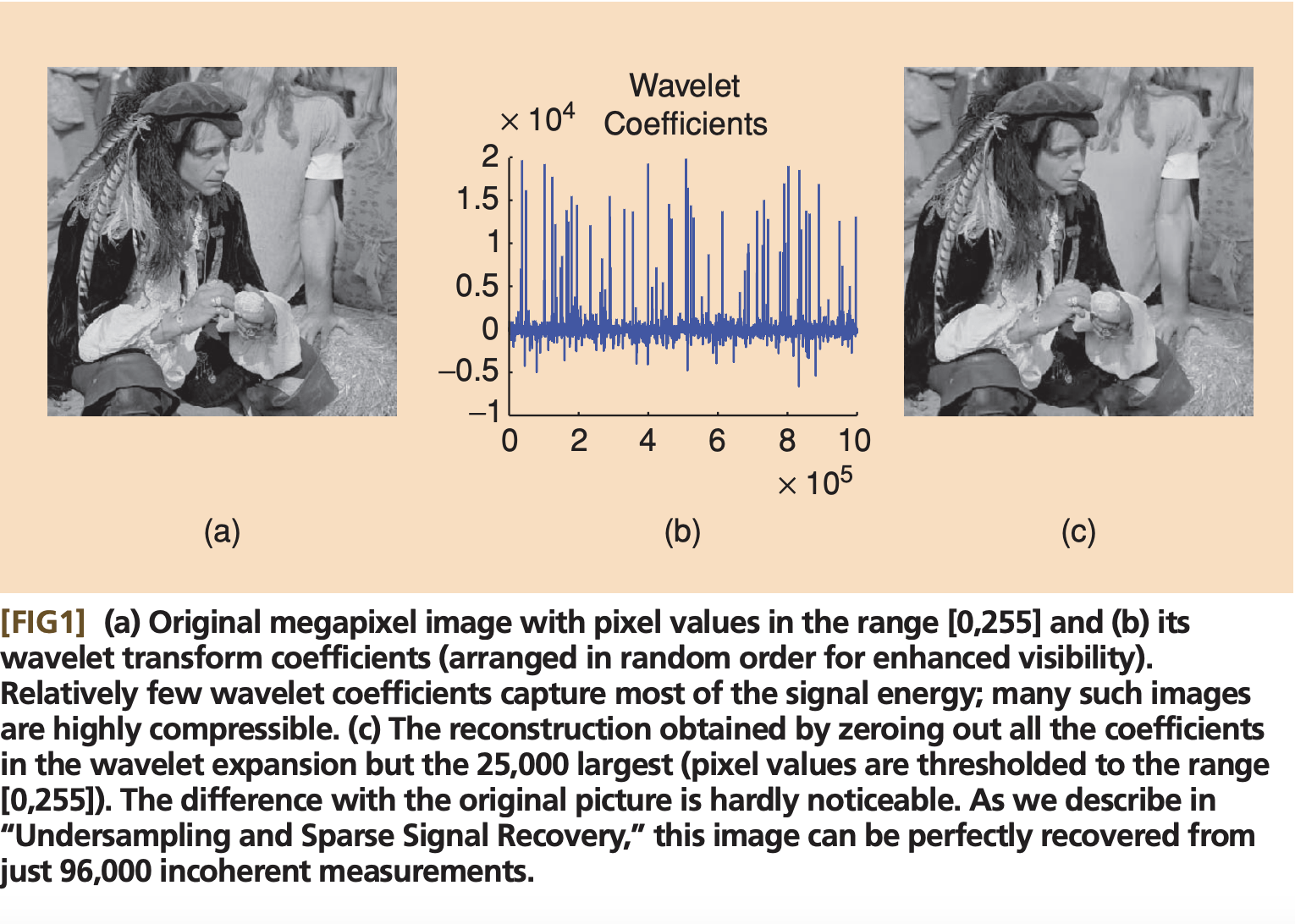
- \( f(t) \) - яркость t-ого пикселя в строке
- \( x_i \) - амплитуда i-го вейвлета
- \( \psi_i(t) \) - i-ый вейвлет Хаара или Даубеши
- \( \Phi \) - например, noiselet
Теорема 1
The exact formulation of Theorem 1 is probabilistic: set a small enough probability δδ, e.g. δ=0.001δ=0.001.
Then with probability not less than 1-δδ the exact recovery of SS-sparse vector xx with a sensing matrix AA is exact, if the number of measurements n≥C⋅S⋅μ2(A)⋅(logN−logδ)\( n \ge Const \cdot \mu^2(A) \cdot S \cdot \log N \).
Here:
- nn is the number of measurements required
- NN is the size of our ambient space
- SS is the maximum number of non-zero coordinates in the vector xx we strive to recover (this number is called sparcity)
- AA is our sensing matrix
-
μ(A)=maxk,j∣Ak,j∣μ(A) = \( \max_{k,j} | A_{k,j} | \) is a bit tricky, it is a quantity called incoherence
Signal incoherence
To understand why signal incoherence is important, let us consider a perfectly bad sensing matrix: let each row of our matrix be a Dirac’s delta, i.e. every measurement measures just a single coordinate of our data vector. How many measurements will it take to recover all the vector coordinates more or less reliably?
This is a coupon collector’s problem: on average N⋅logNN⋅logN measurements will be required to measure every single one of NN coordinates of our data vector.
In this case our sensing matrix is called perfectly coherent: all the “mass” of our measurement is concentrated in a single coordinate. Incoherent measurements matrices, on the other hand, are those that have their mass spread evenly. Note that we impose a condition that l2l2 norm of each vector of the sensing matrices is limited down to N.
Examples of incoherent and coherent sensing matrices
- Dirac’s delta - poor sensing matrix, coherent, see coupon collector problem
- Bernoulli random matrix - an incoherent sensing matrix
-
Gaussian random matrix - another incoherent sensing matrix
-
(possibly incomplete) Fourier Transform matrix - even better sensing matrix
-
random convolution - good sensing matrix (incoherence can be seen in Fourier domain)
See lecture by Emmanuel Candes.
Sensing matrix as a product of measurement matrix and sparsity inducing matrix
In practice sensing matrix AA is a bit constrained.
First, its rows are supposed to have an L2 norm of NN. With this constraint μ(A)μ(A) varies in range 1 to NN. If the “mass” is evenly spread between rows of AA, the matrix is incoherent and is great for compressed sensing. If all the “mass” is concentrated in 1 value, the matrix is highly coherent, and we cannot get any advantage from compressed sensing.
Second, the sensing matrix of measurements cannot be arbitrary, it is determined by the physical nature of measurement process. Typical implementation of the measurement matrix is a Fourier transform matrix.
Third, our initial basis might not be the one, where the signal is sparse.
Sensing matrix as a product of measurement matrix and sparsity inducing matrix
Hence, we might want to decompose our matrix AA into a product of two matrices: measurement matrix and sparsity basis matrix: A=ΦΨA=ΦΨ.
For instance, consider one vertical line of an image. The image itself is not sparse. However, if we applied a wavelet transform to it, in the wavelet basis it does become sparse. Hence, ΨΨ matrix is the matrix of wavelet transform. Now, ΦΦ is the measurement matrix: e.g. if you have a digital camera with a CMOS array or some kind of a photofilm, the measurement matrix ΦΦ might be something like a Fourier transform.
Now we can give a new interpretation to our signal incoherence requirement:
μ(A)=maxk,j∣⟨ϕk,ψj⟩∣μ(A)= \(\max_{k,j} \langle \phi_k, \psi_j \rangle \)
This means that every measurement vector (e.g. Fourier transform vector) should be “spread out” in the sparsity-inducing basis, otherwise the compressed sensing magic won’t work. For instance, if l2-norm of our sensing matrix vectors is fixed to be N \asdfasdfasdfasdf, if all the vector values are 0, and one value is N\( \sqrt{N} \), the sensing magic won’t work, as all the “mass” is concentrated in one point. However, if it is spread evenly (e.g. all the coordinates of each vector have an absolute value of 1), that should work perfectly, and the required number of measurements nn would be minimal.
Теорема 1: шаги доказательства
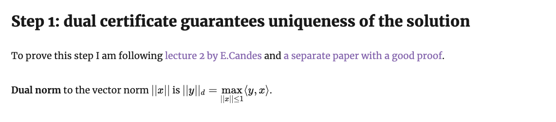
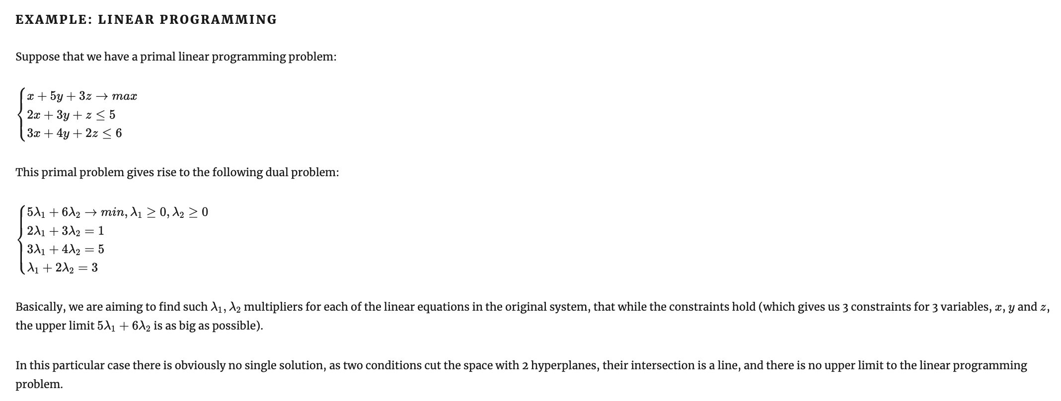
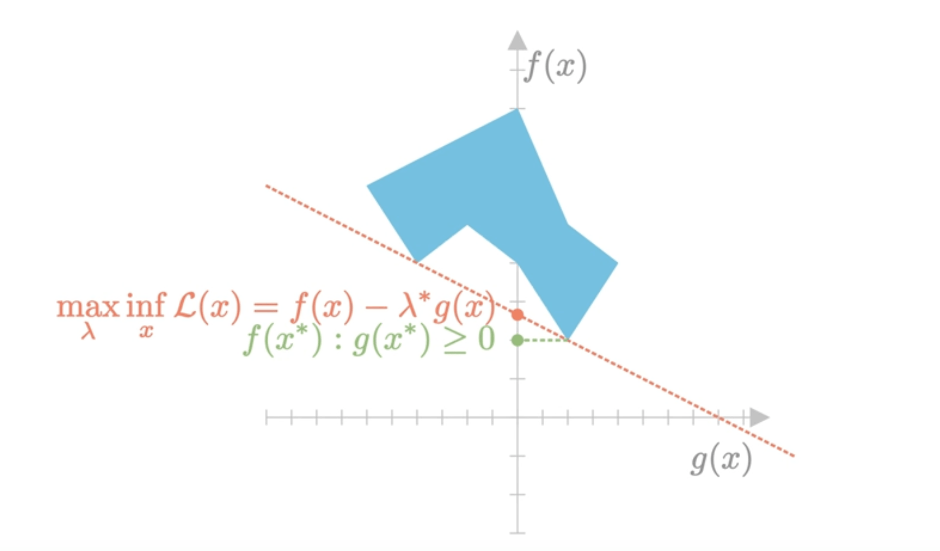
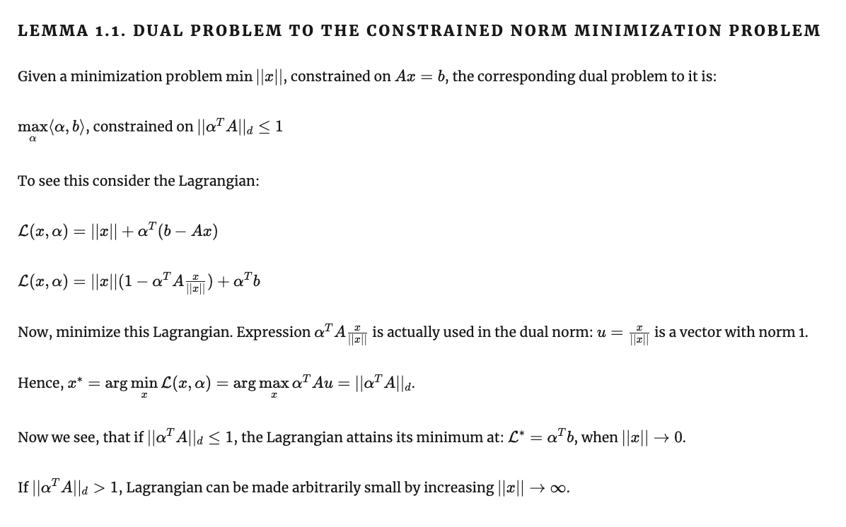
Шаг 1: прямая и двойственная задачи Лагранжа;
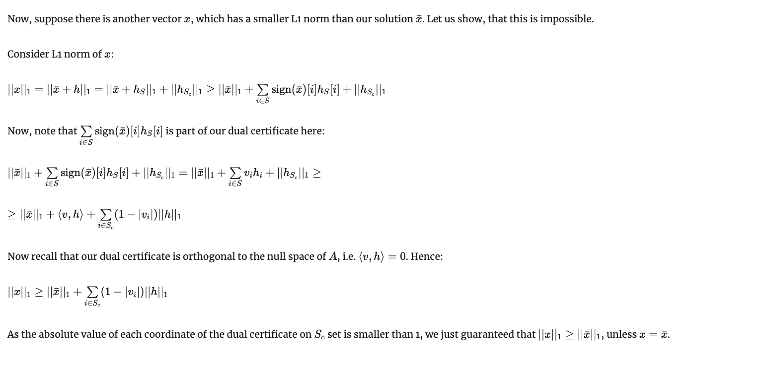
Поскольку регрессия с l1-регуляризацией - выпуклая задача, duality gap = 0. Значит, оптимальному решению прямой задачи соответствует решение двойственной задачи. Если мы можем его предъявить, мы доказали, что соответствующее решение прямой задачи оптимально.
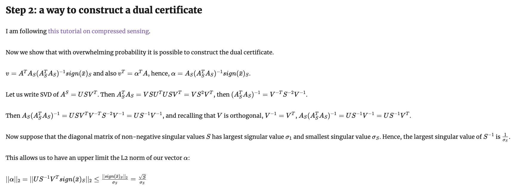
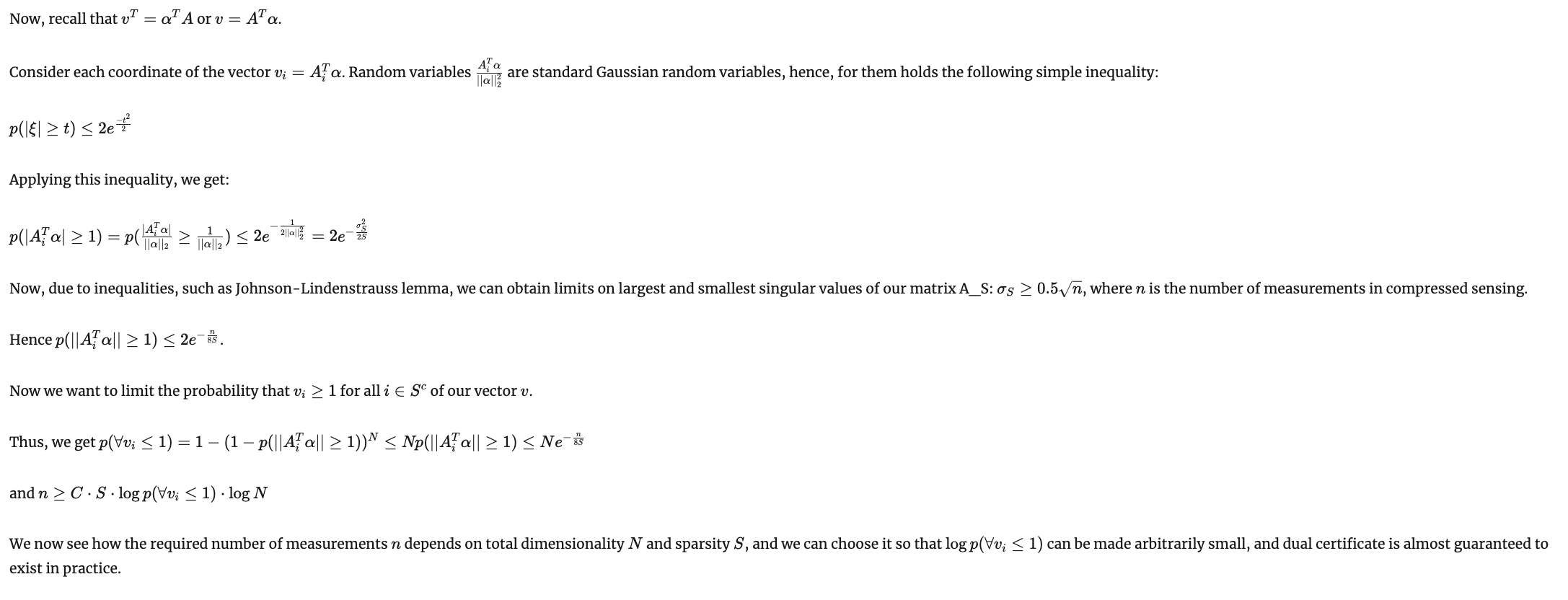
Шаг 2: способ сконструировать сертификат.
Теорема 1: шаг 1
Теорема 1: шаг 1
Что такое прямая и двойственная проблемы Лагранжа
Теорема 1: шаг 1
Что такое прямая и двойственная проблемы Лагранжа
Теорема 1: шаг 1
Теорема 1: шаг 1
Теорема 1: шаг 1
Теорема 1: шаг 1
Теорема 1: шаг 1
Теорема 1: шаг 1
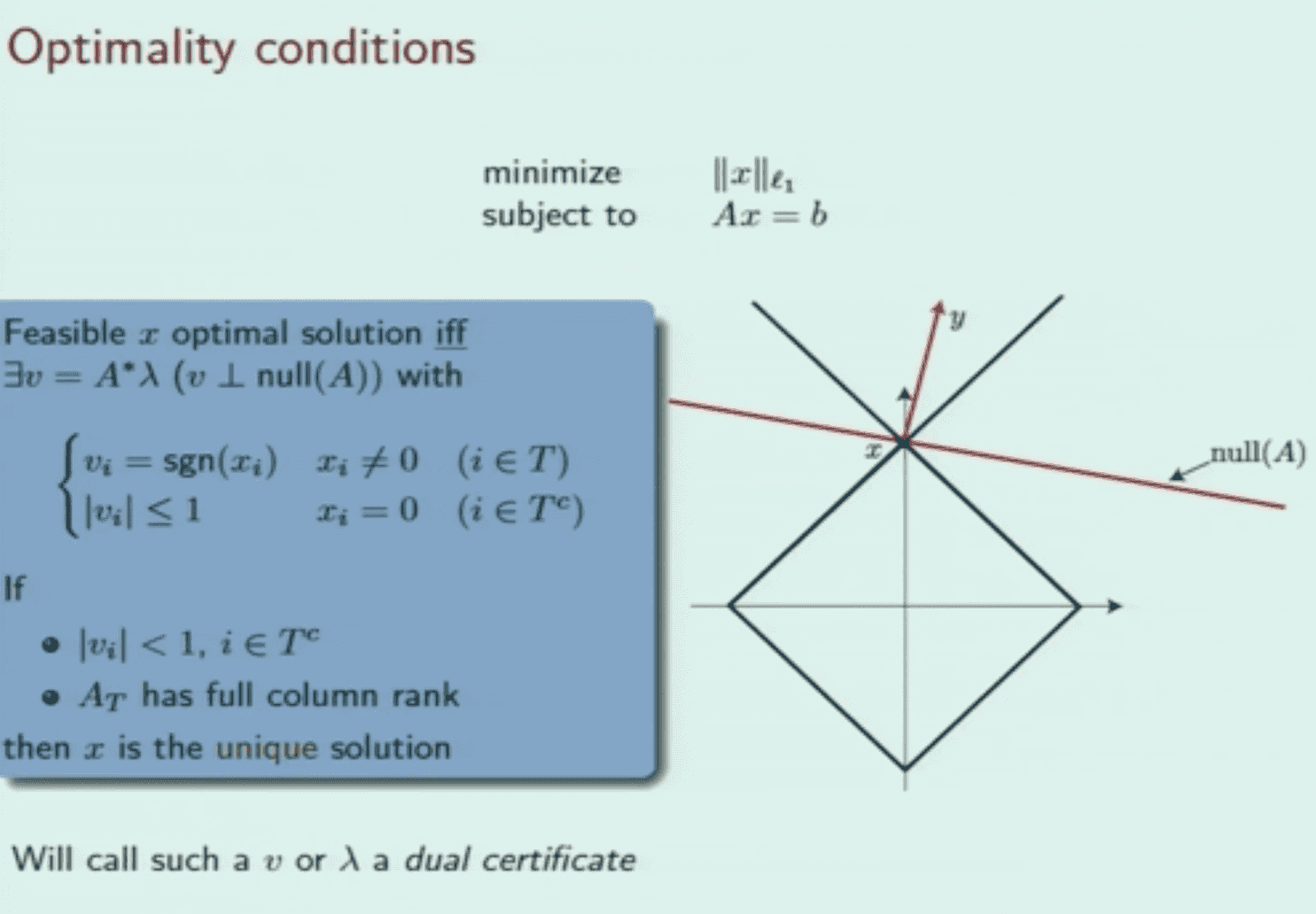
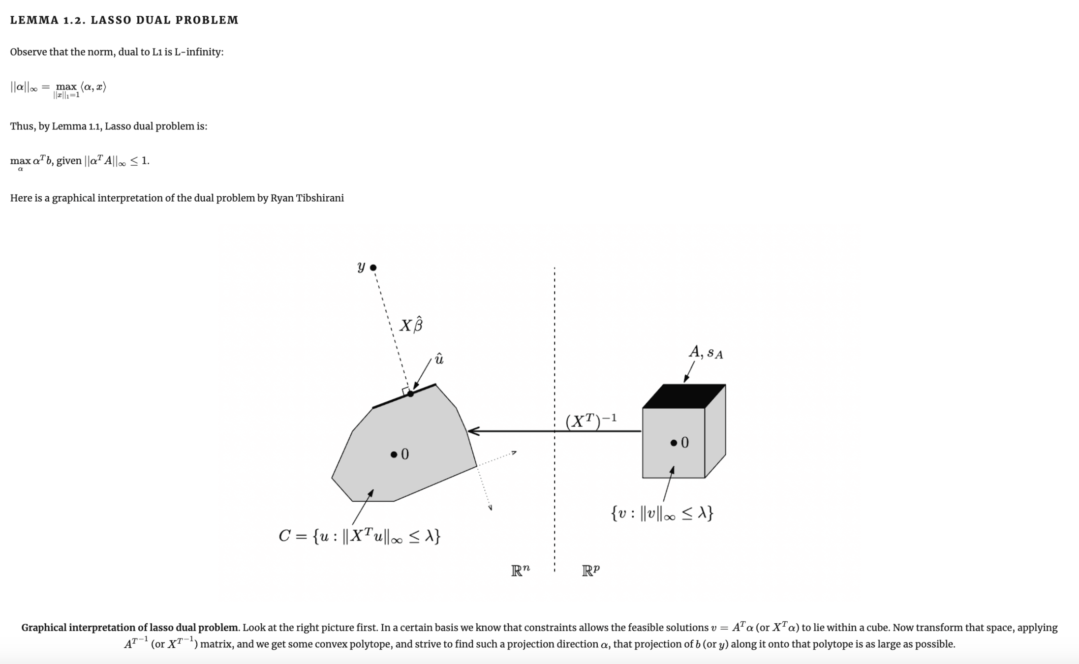
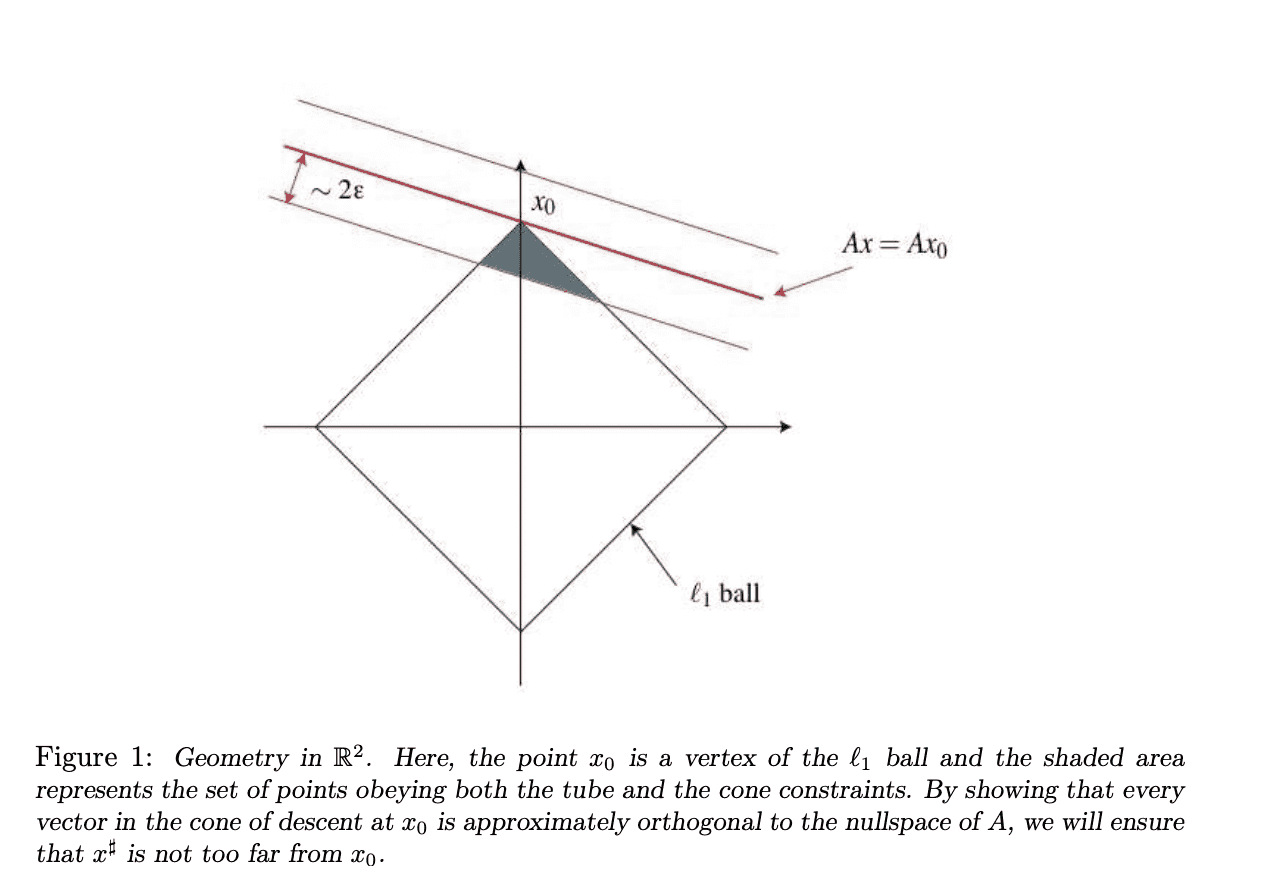
Slide from Cambridge lectures of E.Candes. Image displays a 2D case of our problem with L1 ball, null space of AA operator and vv dual certificate vector.
Теорема 1: шаг 1
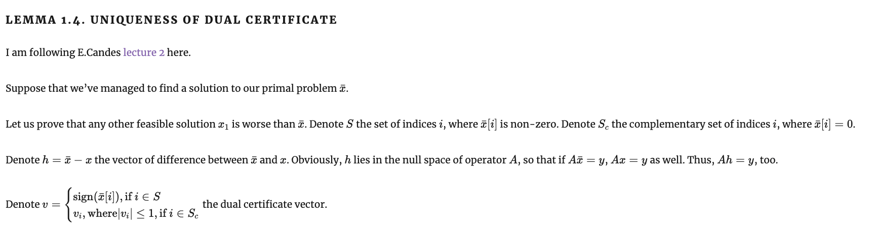
Теорема 1: шаг 2
Теорема 1: шаг 2
Теоремы 2 и 3
Теоремы 2 и 3
Теоремы 2 и 3
Johnson-Lindenstrauss theorem
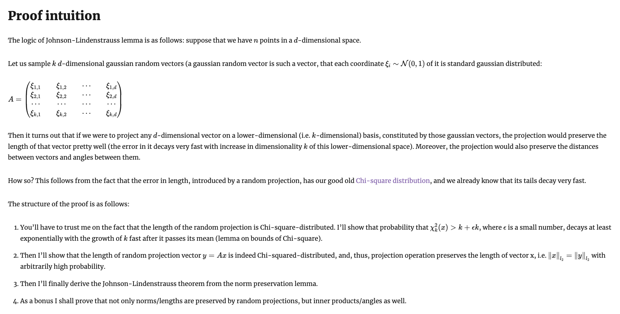
Johnson-Lindenstrauss theorem
Johnson-Lindenstrauss theorem
Johnson-Lindenstrauss theorem
Johnson-Lindenstrauss theorem
Johnson-Lindenstrauss theorem
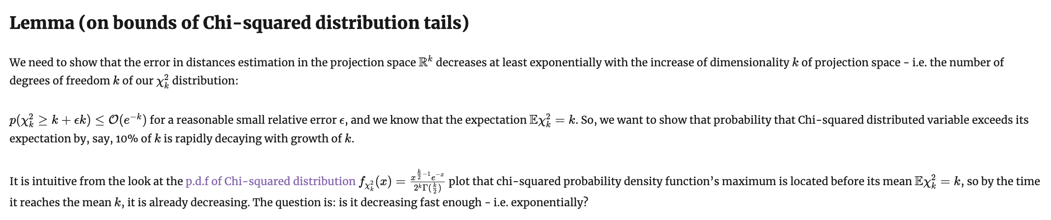
Johnson-Lindenstrauss theorem
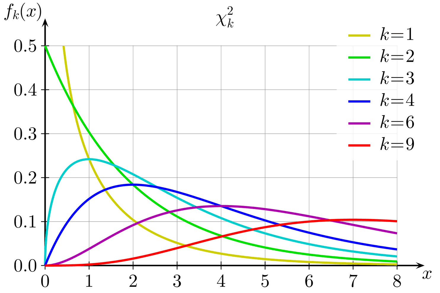
Johnson-Lindenstrauss theorem
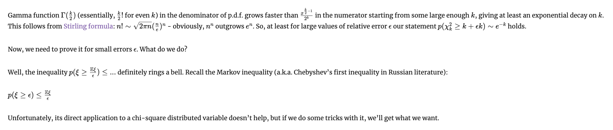
Johnson-Lindenstrauss theorem
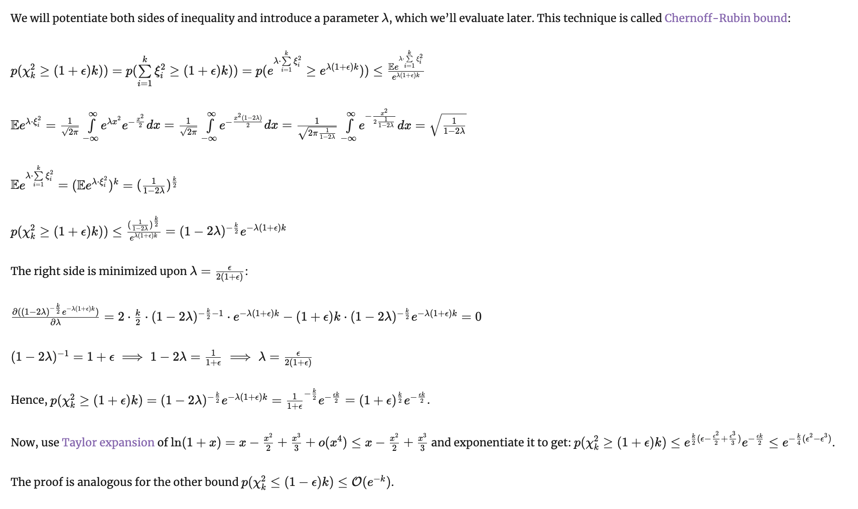
Johnson-Lindenstrauss theorem
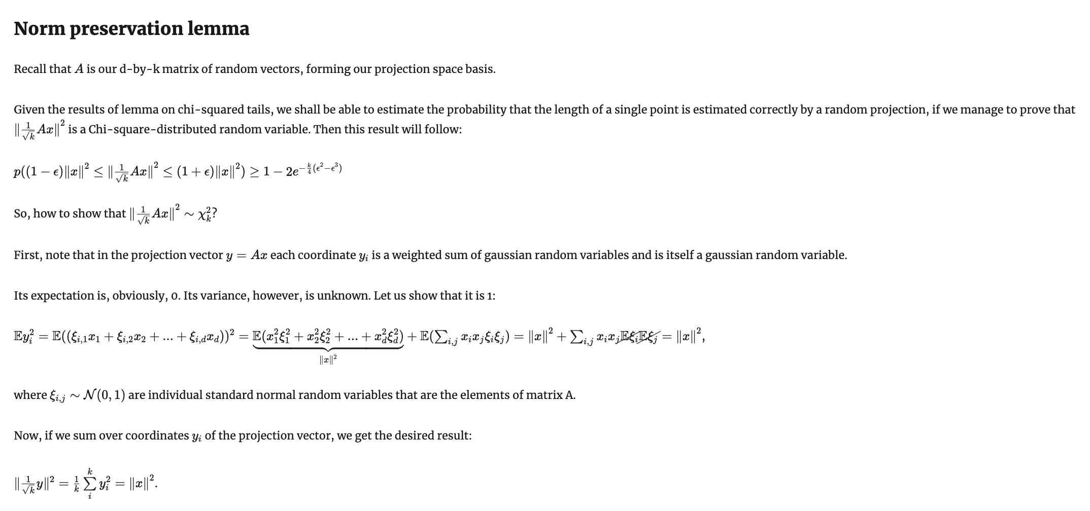
Johnson-Lindenstrauss theorem
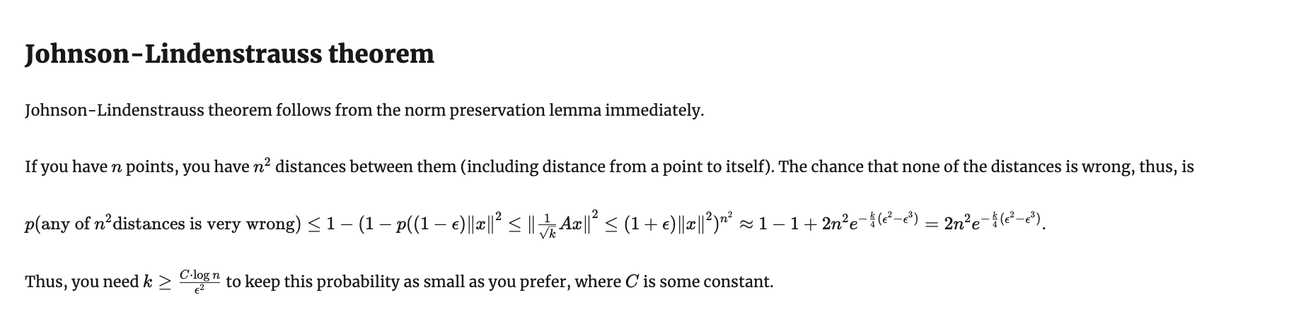
Johnson-Lindenstrauss theorem
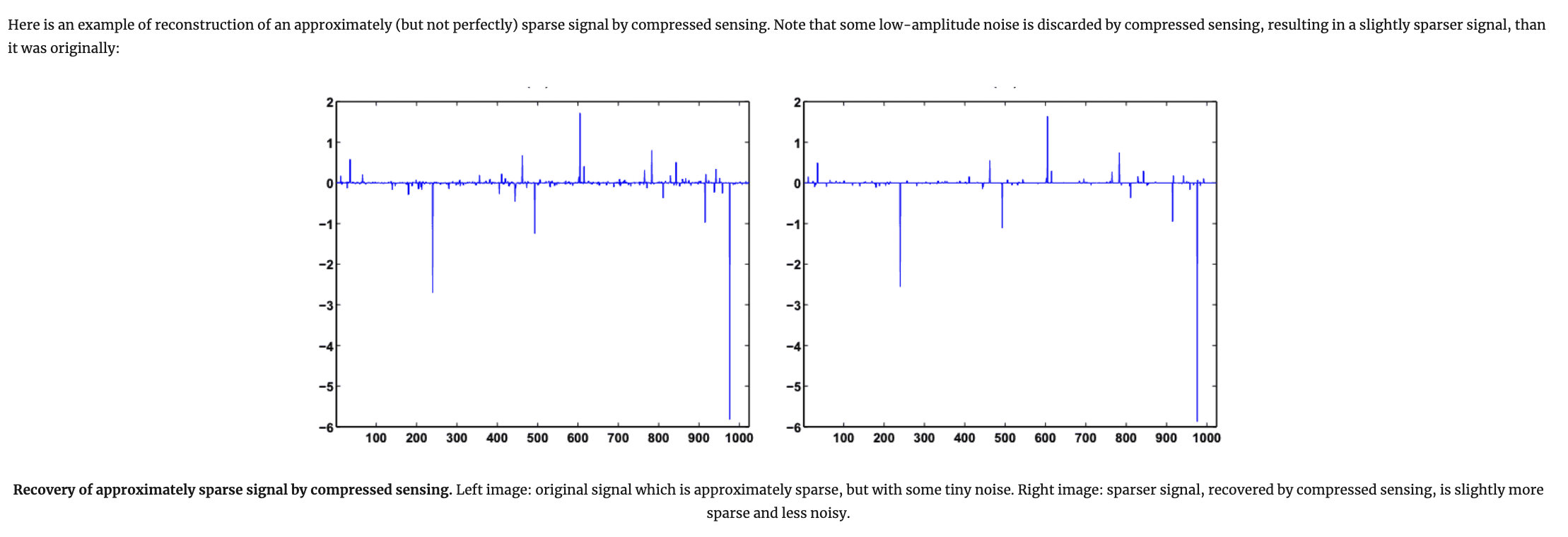
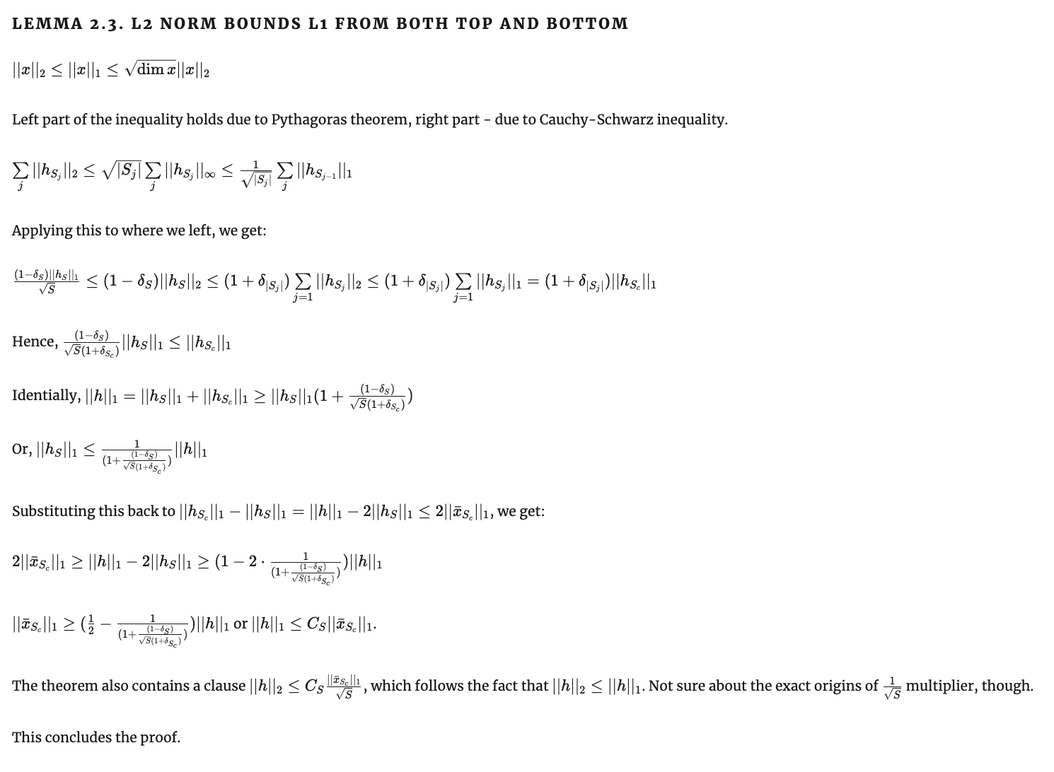
Теорема 2 compressed sensing: устойчивость к шуму в разреженном сигнале
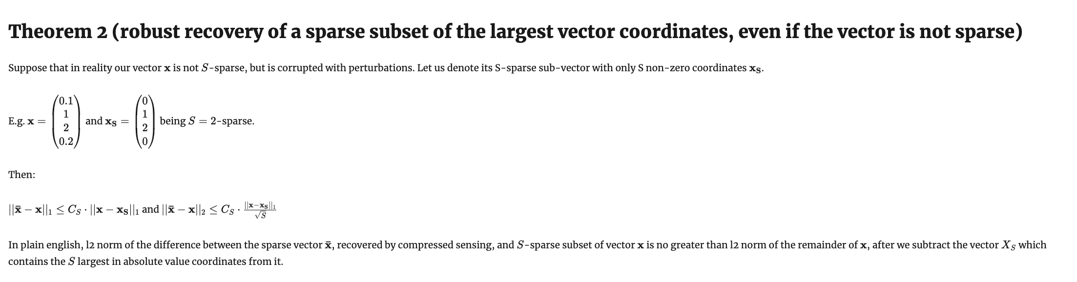
Теорема 2
Теорема 2
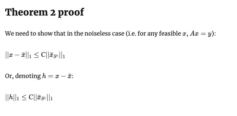
Теорема 2
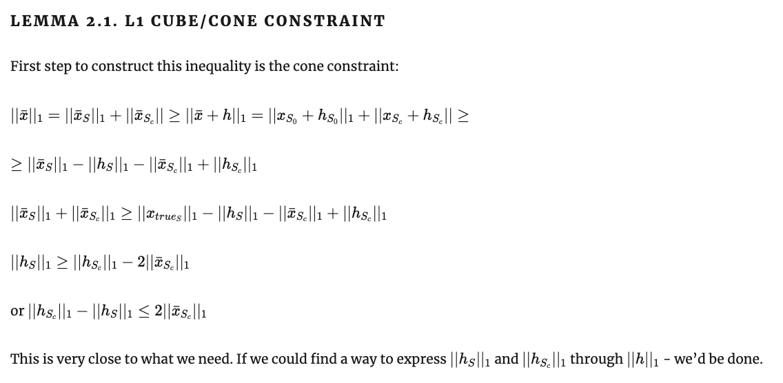
Теорема 2
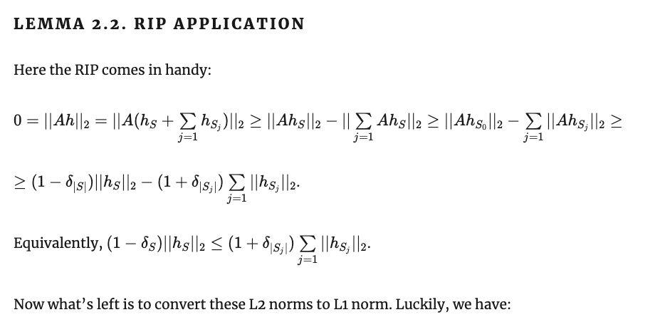
Теорема 2
Теорема 3 compressed sensing: устойчивость к шуму измерений
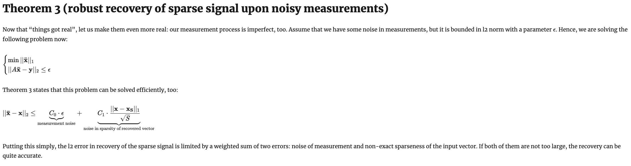
Теорема 3
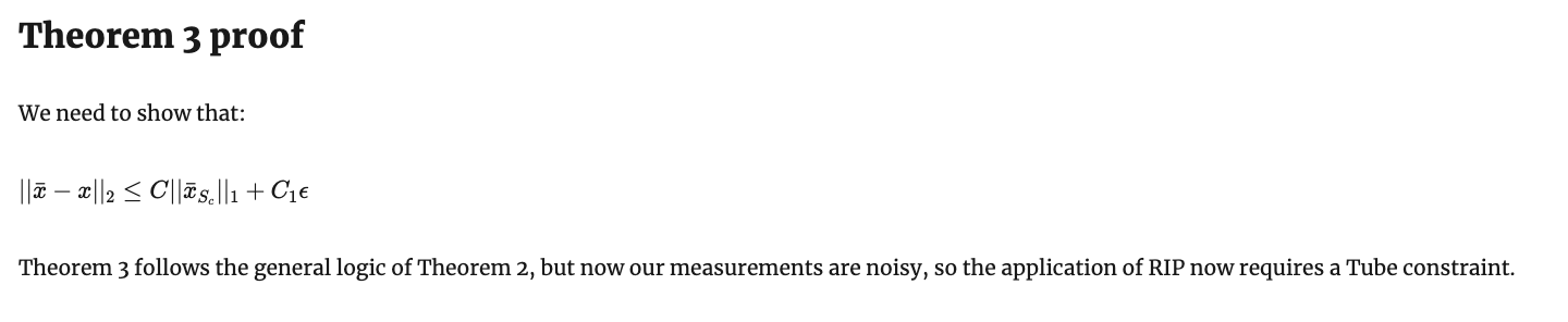
Теорема 3
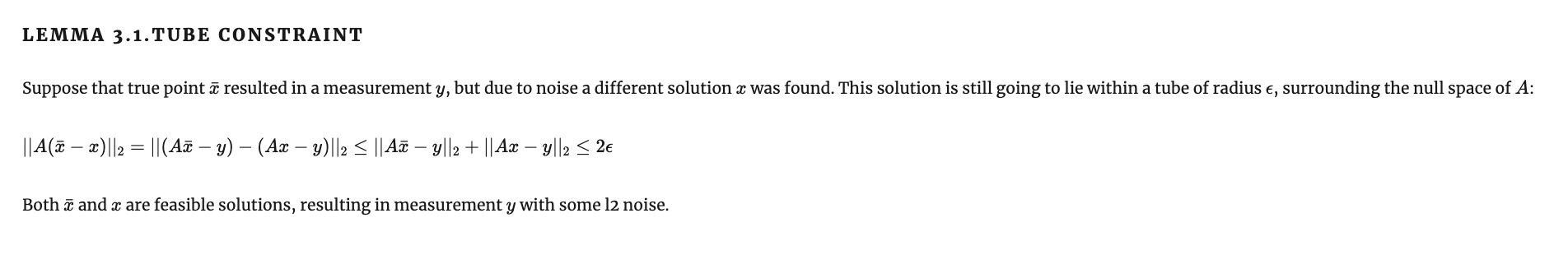
Теорема 3
Теорема 3
Trace (nuclear) Norm
Можно минимизировать не только L1-норму векторов, но и L1-норму разных интересных объектов. Например, вектора собственных или сингулярных значений. Там можно добиться аппроксимации матрицы матрицей низкого ранга.
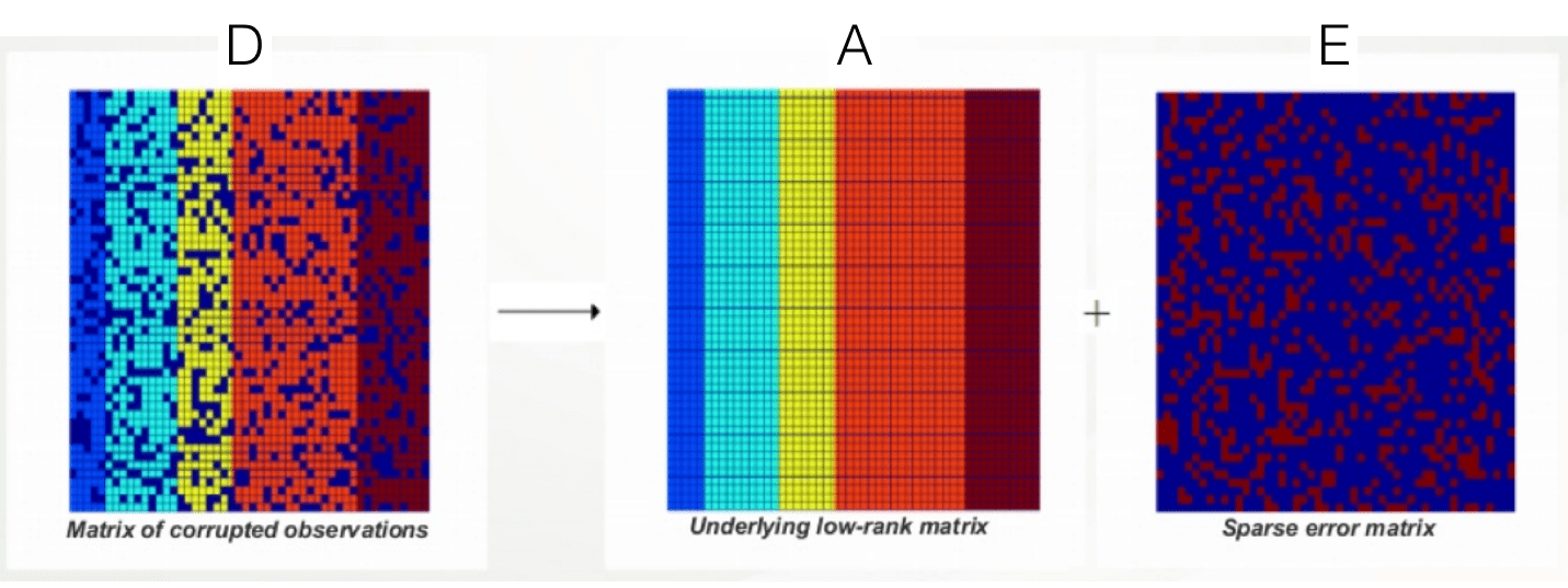
Robust PCA
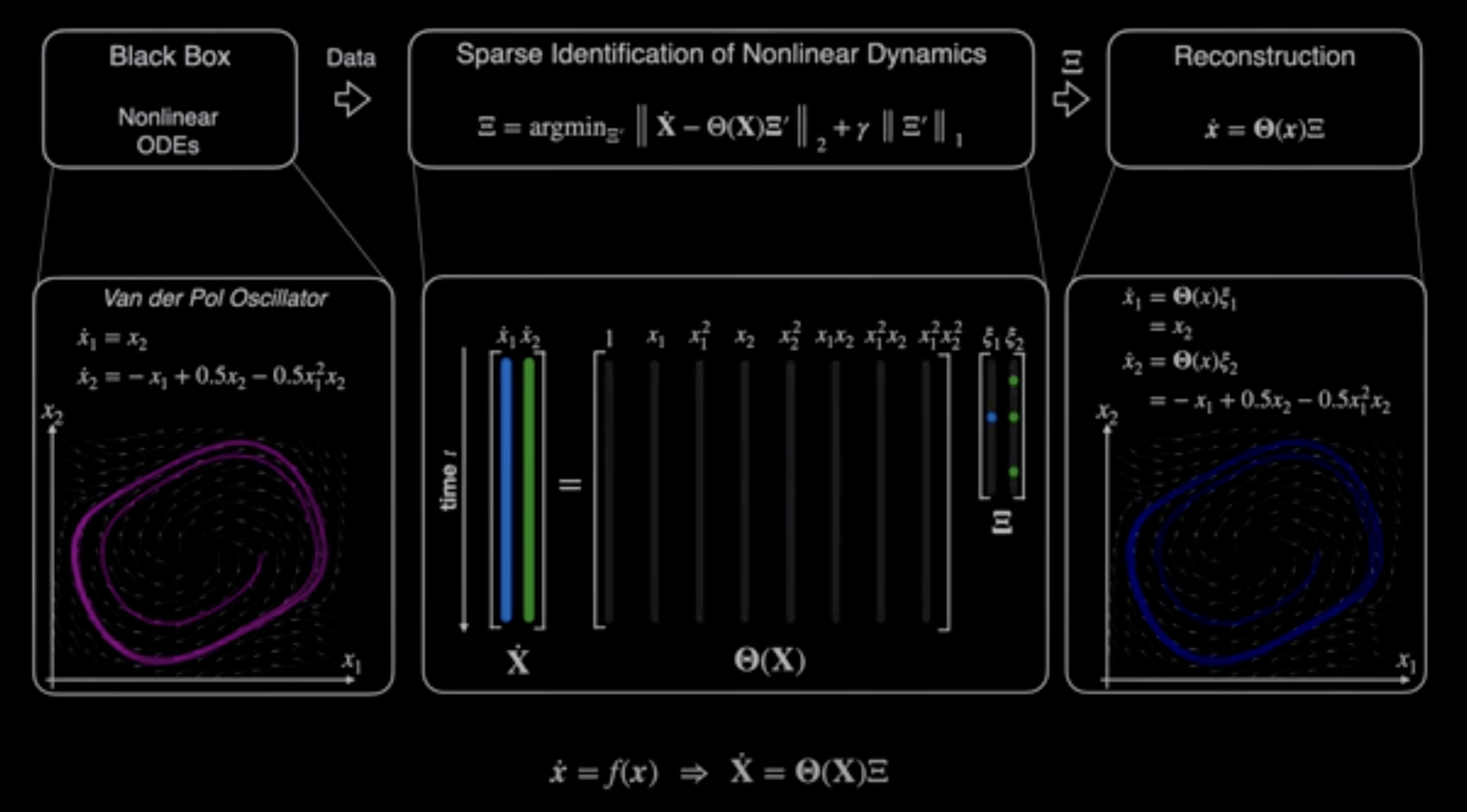
Sparse identification of nonlinear dynamics (SINDy)
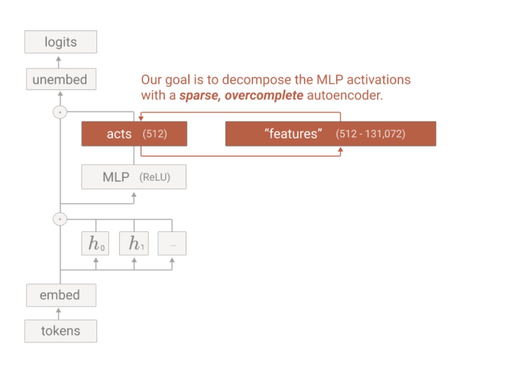
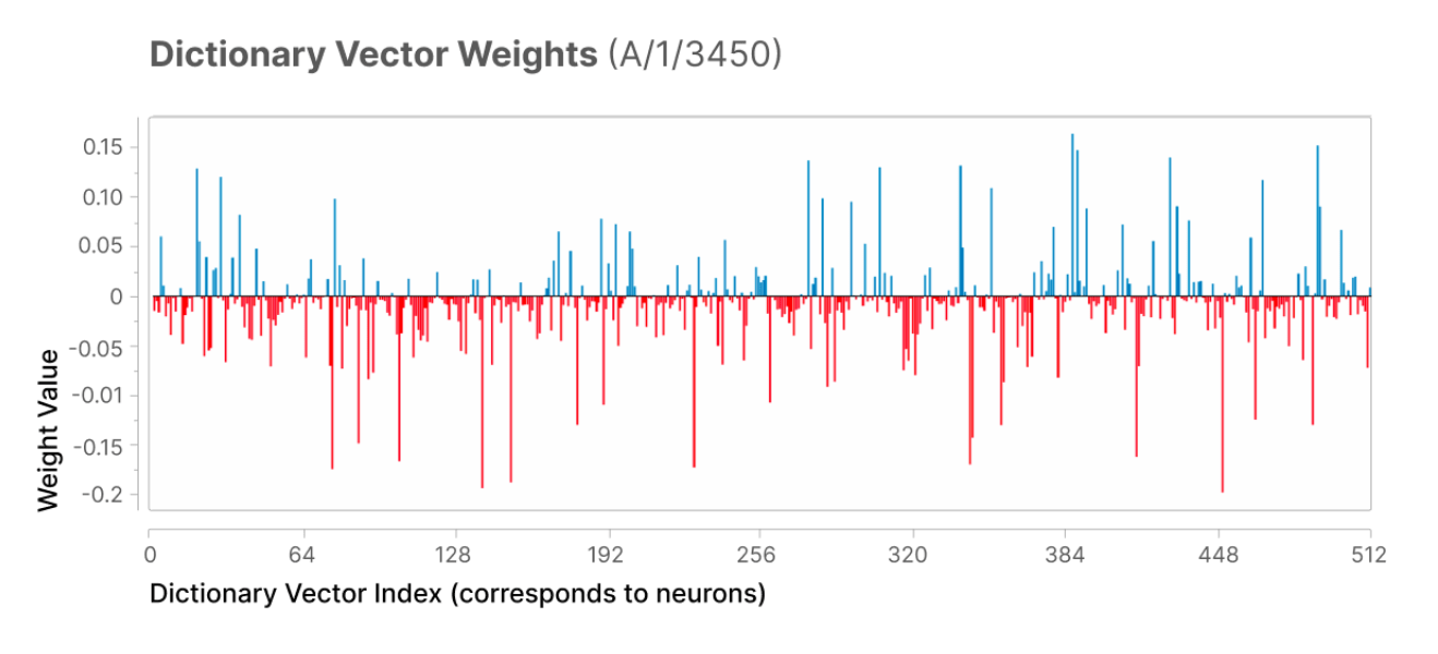
Sparse autoencoders
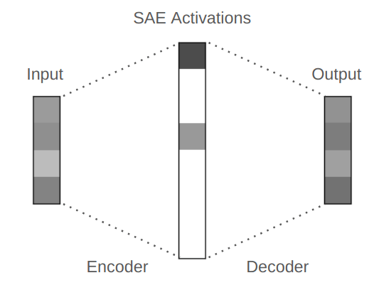
Sparse autoencoders