1o Meeting of Postdocs at IME-USP
Victor Sanches Portella
April, 2025
ime.usp.br/~victorsp
The Mathematics of
Learning
Online
Private
and
Who am I?
Postdoc supervised by prof. Yoshiharu Kohayakawa
ML Theory
Optimization
Randomized Algs
Optimization


My interests according to a student:
"Crazy Algorithms"
Online Learning
Prediction with Expert's Advice
Player
Adversary
\(n\) Experts
0.5
0.1
0.3
0.1
Probabilities
1
-1
0.5
-0.3
Costs
Player's loss:
Adversary knows the strategy of the player


Measuring Player's Perfomance
Total player's loss
Can be = \(T\) always
Compare with offline optimum
Almost the same as Attempt #1
Restrict the offline optimum
Attempt #1
Attempt #2
Attempt #3
Loss of Best Expert
Player's Loss
Goal:
Example
Cummulative Loss
Experts
Why Learning with Experts?
Boosting in ML
Understanding sequential prediction & online learning
Universal Optimization

TCS, Learning theory, SDPs...


Some Work of Mine

Algorithms design guided by
PDEs and (Stochastic) Calculus tools
Modeling Online Learning in Continuous Time

Analysis often becomes clean
Sandbox for design of optimization algorithms
Gradient flow is useful for smooth optimization
Key Question: How to model non-smooth (online) optimization in continuous time?
Why go to ?
continuous time
Modeling Adversarial Costs in Continuous Time
Total loss of expert \(i\):


Useful perspective: \(L(i)\) is a realization of a random walk
realization of a Brownian Motion
Probability 1 = Worst-case
Discrete Time
Continuous Time
Differential Privacy
What do we mean by "privacy" in this case?
Informal Goal: Output should not reveal (too much) about any single individual
Not considering protections against security breaches
Output
Data Analysis
Output should have information about the population
This has more to do with "confidentiality" than "privacy"
Real-life example - Netflix Dataset

Differential Privacy
Output 1
Output 2
Indistinguishible
Differential Privacy
Anything learned with an individual in the dataset
can (likely) be learned without

\(\mathcal{M}\) needs to be randomized to satisfy DP
Adversary with full information of all but one individual can infer membership
Differential Privacy (Formally)
Any pair of neighboring datasets: they differ in one entry
\(\mathcal{M}\) is \((\varepsilon, \delta)\)-Differentially Private if
Definition:
\((\varepsilon, \delta)\)-DP
\(\varepsilon \equiv \) "Privacy leakage", in theory constant \(\leq 1\)
\(\delta \equiv \) "Chance of failure", usually VERY small
An Example: Computing the Mean
Goal:
\((\varepsilon, \delta)\)-DP such that approximates the mean of \(x_i\)'s
Algorithm:
Gaussian or Laplace noise

with
Some of my Work - Covariance Estimation
Unknown Covariance Matrix
\((\varepsilon, \delta)\)-differentially private \(\mathcal{M}\) to estimate \(\Sigma\)
on \(\mathbb{R}^d\)
There are
ARE THEY OPTIMAL?
Previous results:
Our results:
YES... under some artificial restrictions
YES!
A Lower Bound Strategy
Assume \(\mathcal{M}\) is
accurate
There is high correlaton between output and input
Feed to \(\mathcal{M}\) a marked input \(X\)
\((\varepsilon,\delta)\)-DP implies
Opposing Conditions
Correlation is bounded
Stokes' Theorem (!?)
Stein's Lemma (!)

Online meets Private
Online and Private Learnability are Equivalent
Bounded in terms of VC Dimension of
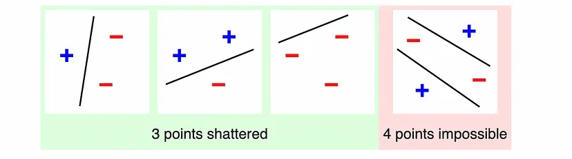
PAC Learning
How many examples
from set of hyptheses
to "learn"
Online and Private Learnability are Equivalent
PAC Learning
How many examples
from set of hyptheses
to "learn"
Private
with differential privacy
Bounded in terms of Littlestone Dimension of
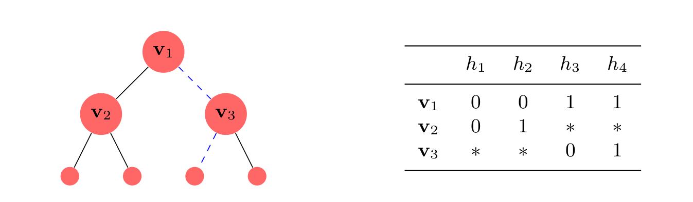
Characterizes
ONLINE LEARNABILITY
Tighter bounds?
Algorithmic implications?
Circumvent OL?
Online Learning, Privately
We need to release information at every round
But changes are usually incremental
Can we do better than naive algorithms?

Some Applications
ML Training
Synthetic Data Generation
Boosting
How can we make
Online Learning
private?
Online Algorithms
Final Remarks
Differential Privacy is a formal definition of private computation
Online Learning is a powerful learning theory framework
Both are connected?!
Thanks!
Many interesting questions
Better investigate the connections of OL and DP
Find new algorithms and limits for Online DP
DP and Other Areas of ML and TCS
Online Learning
Adaptive Data Analysis and Generalization in ML
Robust statistics


Proof uses Ramsey's Theory :)
Backup Slides
Take Away from Examples
Privacy is quite delicate to get right
Hard to take into account side information
"Anonymization" is hard to define and implement properly
Different use cases require different levels of protection
Real-life example - NY Taxi Dataset

Summary: License plates were anonymized using MD5
Easy to de-anonymize due to lincense plate structure

By Vijay Pandurangan
https://www.vijayp.ca/articles/blog/2014-06-21_on-taxis-and-rainbows--f6bc289679a1.html
An Example: Computing the Mean
Goal:
is small
\((\varepsilon, \delta)\)-DP such that approximates the mean:
Algorithm:
Gaussian or Laplace noise
with
OPTIMAL?
Theorem
\(Z \sim \mathcal{N}(0, \sigma^2 I)\) with
\(\mathcal{M}\) is \((\varepsilon, \delta)\)-DP and
The Advantages of Differential Privacy
Worst case: No assumptions on the adversary
Immune to post-processing: Any computation on the output can only improve the privacy guarantees
Composable: DP guarantees of different algorithms compose nicely, even if done in sequence and adaptively
Online Algorithms in General
Online Algorithms:
data is processes one piece at a time
Online Learning
Streaming
???
Fingerprinting Codes
Avoiding Pirated Movies via Fingerprinting

Movie may leak!

Movie Owner
Can we detect one ?
?

Idea: Mark some of the scenes (Fingerprinting)

Fingerprinting Codes
\(d\) scenes
\(n\) copies of the movie
1 = marked scene
0 = unmarked scene
Code usually randomized
We can do with \(d = 2^n\). Can \(d\) be smaller?
Example of pirating:
\(0\) or \(1\)
\(0\) or \(1\)
Only 1
Goal of fingerprinting
Given a copy of the movie, trace back one
with probability of
false positive \(o(1/n)\)
Fingerprinting Codes for Lower Bounds
Assume \(\mathcal{M}\) is
accurate
Adversary can detect some \(x_i\)
with high probability
Feed to \(\mathcal{M}\) a marked input \(X\)
\((\varepsilon,\delta)\)-DP implies adversary detects \(x_i\) on \(\mathcal{M}(X')\) with
\(X' = X - \{x_i\} + \{z\}\)
CONTRADICTION
FP codes with \(d = \tilde{O}(n^2)\)
Output -> Pirated Movie
Breaks False Positive Guarantee
[Tardos '08]
The Good, The Bad, and The Ugly of Codes
The Ugly:
Black-box use of FP codes makes it hard to adapt it to
other settings
The Bad:
Very restricted to binary inputs
The Good:
Leads to optimal lower bounds for a variety of problems
Fingerprinting Lemmas
Fingerprinting Lemmas
Idea: For some distribution on the input,
the output is highly correlated with the input
Lemma (A 1D Fingerprinting Lemma, [Bun, Stein, Ullman '16])
\(\mathcal{M} \colon [-1,1]^n \to [-1,1]\)
\(p \sim \mathrm{Unif}(\{-1,1\})\)
\(x_1, \dotsc, x_n \in \{\pm 1\}\) random such that \(\mathbb{E}[x_i] = p\)
"Correlation" between \(x_i\) and \(\mathcal{M}(X)\)
\(\mathcal{A}(x_i, \mathcal{M}(X))\)
Fingerprinting Lemma - Picture
If \(\mathcal{M}\) is accurate
large
If \(z\) indep. of \(X\)
small
Depends on distribution of \(X\) and \(p\)
From 1D Lemma to a Code(-Like) Object
Fingerprinting Lemma leads to a kind of fingerprinting code
Bonus: quite transparent and easy to describe
Key Idea: Make \(\tilde{O}(n^2)\) independent copies
\(\mathcal{M} \colon ([-1,1]^d)^n \to [-1,1]\)
\(p \sim \mathrm{Unif}(\{-1,1\})^d\)
\(x_1, \dotsc, x_n \in \{\pm 1\}^d\) random such that \(\mathbb{E}[x_i] = p\)
for \(d = \Omega(n^2 \log n)\)
\(\mathcal{A}(x_i, \mathcal{M}(X))\)
From Lemma to Lower Bounds
If \(\mathbb{E}(\lVert \mathcal{M}(X) - p\rVert_2^2) \leq d/6\)
If \(\mathcal{M}\) is accurate, correlation is high
If \(\mathcal{M}\) is \((\varepsilon, \delta)\)-DP, correlation is low
\(\mathcal{A}(x_i, \mathcal{M}(X))\)
Extension to Gaussian Case
Lemma (Gaussian Fingerprinting Lemma)
\(\mathcal{M}\colon \mathbb{R}^n \to \mathbb{R}\)
\(\mu \sim \mathcal{N}(0, 1/2)\)
\(x_1, \dotsc, x_n \sim \mathcal{N}(\mu,1)\)
One advantage of lemmas over codes:
Easier to extend to different settings
Implies similar lower bounds for privately estimating the mean of a Gaussian
Lower Bounds for Gaussian
Covariance Matrix Estimation
Work done in collaboration with Nick Harvey

Roadblocks to Fingerprinting Lemmas
Unknown Covariance Matrix
on \(\mathbb{R}^d\)
To get a Fingerprinting Lemma, we need random \(\Sigma\)
Most FPLs are \(d = 1\), and then use independent copies
leads to limited lower bounds for covariance estimation
[Kamath, Mouzakis, Singhal '22]
We can use diagonally dominant matrices, but
0 has error \(O(1)\)
Can't lower bound accuracy of algorithms with \(\omega(1)\) error
Diagonal
Off-diagonal
Our Results
Theorem
For any \((\varepsilon, \delta)\)-DP algorithm \(\mathcal{M}\) such that
and
we have
Our results covers both regimes
Nearly highest reasonable value
[Kamath et al. 22]
Previous lower bounds required
[Narayanan 23]
OR
Main Contribution: Fingerprinting Lemma without independence
Which Distribution to Use?
Wishart Distribution
Our results use a very natural distribution:
\(d \times 2d\) random Gaussian matrix
Natural distribution over PSD matrices
Entries are highly correlated
A Different Correlation Statistic

A Peek Into the Proof for 1D
Lemma (Gaussian Fingerprinting Lemma)
\(\mu \sim \mathcal{N}(0, 1/2)\)
\(x_1, \dotsc, x_n \sim \mathcal{N}(\mu,1)\)
Claim 1
Claim 2
Stein's Lemma
Follows from integration by parts
A Peek Into the Proof of New FP Lemma
Fingerprinting Lemma
Need to Lower Bound
\(\Sigma \sim\) Wishart leads to elegant analysis
Stein-Haff Identity
"Move the derivative" from \(g\) to \(p\) with integration by parts
Stokes' Theorem
CombΘ Seminar
for Lower Bounds
Differential Privacy
An Introduction to
Fingerprinting Techniques
and

Victor Sanches Portella
November, 2024
cs.ubc.ca/~victorsp