Hardware Software Co-Design for Efficient Deep Learning Systems

Vinod Ganesan
Dept. of CSE, IIT Madras
Deep Learning is revolutionizing our daily lives



Source: Jeff Dean ISSCC 2020 [1]
[1] Deep Learning Revolution and its Implications for Computer Architecture and Chip Design, ISSCC 2020
The cost of the revolution - Exploding Compute demands
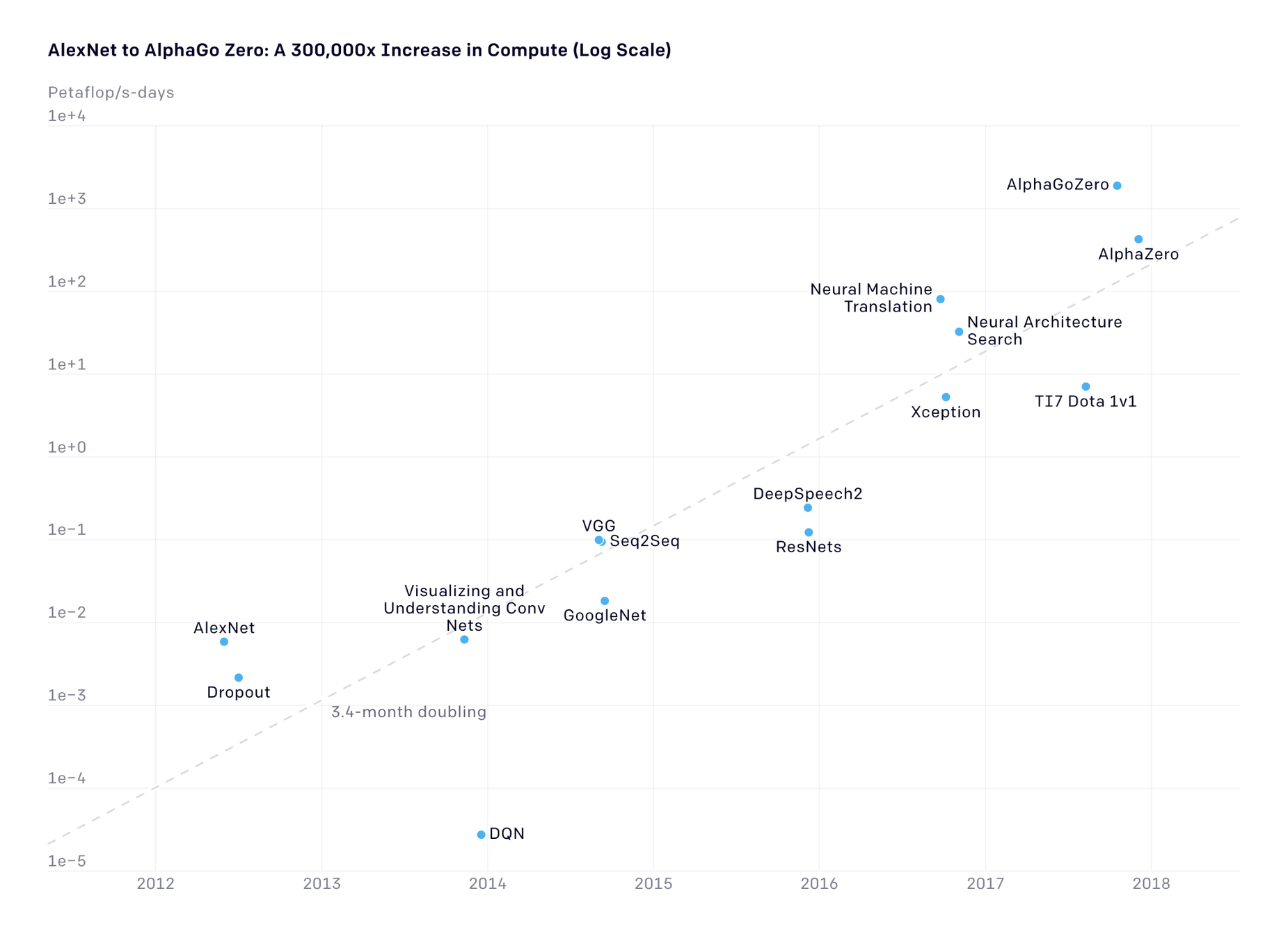
10x/year
Source: OpenAI Blog [1]
Moore's law
There is a huge demand gap
Addressing this problem is vital to sustain the growth trajectory of DL
[1] https://openai.com/blog/ai-and-compute/
Source: OpenAI Blog [1]
Our thesis
Efficient Deep Learning
Efficient Systems
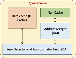
SparseCache
Efficient Design Methodology
Generalizable cost models
Efficient Neural Networks
FuSeConv
DATE 2020
IISWC 2020
DATE 2021
Our thesis
Efficient Deep Learning
Efficient Systems
SparseCache
Efficient Design Methodology
Generalizable cost models
Efficient Neural Networks
FuSeConv
DATE 2020
Motivation
Enabling DNNs on resource-constrained environments is challenging

Area: 0.1-2 \( mm^2 \)
Power: ~100mW
Motivation: What about accelerators?
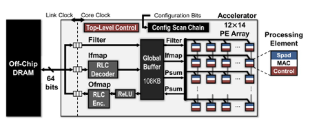
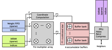
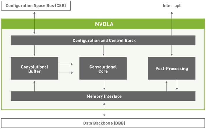
Eyeriss (2016): 12.25 \( mm^2 \)
SCNN (2017): 8 \( mm^2 \)
NVDLA (2017): 5 \( mm^2 \)
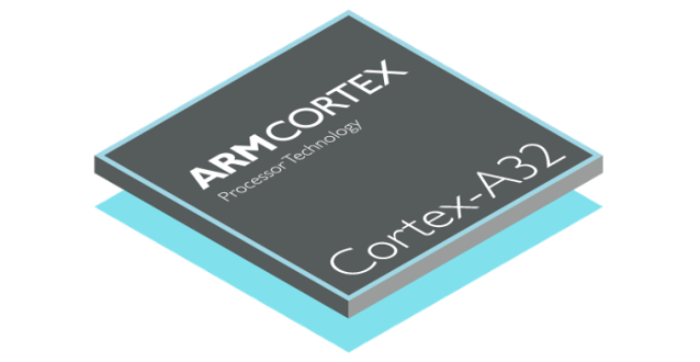
Area: ~0.4 \( mm^2 \)
Very high area requirements!
[1]. Chen et. al, Eyeriss: A Spatial Architecture for Energy-Efficient Dataflow for Convolutional Neural Networks, ISCA 2016
[2]. Parashar et. al, SCNN: An Accelerator for Compressed-sparse Convolutional Neural Networks, ISCA 2017
[3]. http://nvdla.org/
Motivation: Optimizing General Purpose Processors is Vital!

Area: ~0.4 \( mm^2 \)
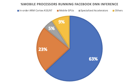
Wu et. al, HPCA 2019 [1]
Key Idea: Develop light-weight micro-architectural extensions for general purpose processors
[1] Wu. et al, Machine Learning at Facebook: Understanding Inference at the Edge, HPCA 2019
Insight: Caches have high miss-rates running DNNs
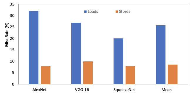
Reducing this miss rate is crucial to improving performance
16KB 4-way Set Associative Cache
Insight: DNNs are highly sparse and pollute the cache
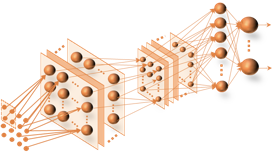

DNN data structures
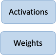

Dynamic Sparsity
Static Sparsity
50.6%
65.6%


Effective Cache Capacity
Miss rate
Performance
Zero values pollute the cache
Key Idea 2: Develop Cache extensions to store zero-valued addresses compactly
Insight: Coarse grained sparsity is preferred
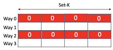
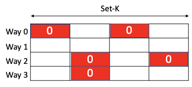


Storing these zero cache-line addresses separately is not sufficient

Key Idea 3: Merge and store contiguous/strided zero-valued cache line addresses compactly
Key Ideas
- Develop lightweight micro-architectural extensions for general-purpose processors to accelerate DL
- Develop cache-extensions to store zero-valued addresses compactly
- Merge and store multiple zero valued addresses in a single entry
Proposal
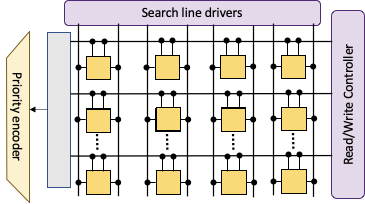
Augment the cache-architecture with a TCAM based "null cache" to store zero valued addresses
Solution: TCAM as a compact storage
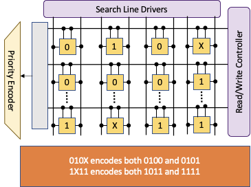
- Ternary Content Addressable Memories are capable of encoding don't cares "X" in addition to 0s and 1s
- Each entry can store multiple contiguous or strided addresses with appropriate "X"s
- Best fit for DNN workloads exhibiting coarse grained sparsity
Challenges with TCAM
- Dynamically identify zero cache-blocks
- Low area and power overhead
- Dynamically identify and merge multiple entries in TCAM
0
1
0
0
4-bit zero-cache line address
Challenges with TCAM
- Dynamically identify zero cache-blocks
- Low area and power overhead
- Dynamically identify and merge multiple entries in TCAM

0
1
0
0
0
0
0
1
Challenges with TCAM
- Dynamically identify zero cache-blocks
- Low area and power overhead
- Dynamically identify and merge multiple entries in TCAM

0
1
0
0
0
0
0
1
0
0
1
0
1
Challenges with TCAM
- Dynamically identify zero cache-blocks
- Low area and power overhead
- Dynamically identify and merge multiple entries in TCAM

0
1
0
0
0
0
0
1
0
0
1
0
X
First Order Merge
Challenges with TCAM
- Dynamically identify zero cache-blocks
- Low area and power overhead
- Dynamically identify and merge multiple entries in TCAM

0
1
0
0
0
0
0
1
0
0
1
0
X
First Order Merge
0
0
0
0
Challenges with TCAM
- Dynamically identify zero cache-blocks
- Low area and power overhead
- Dynamically identify and merge multiple entries in TCAM

0
1
0
0
0
0
0
1
0
0
1
0
X
First Order Merge
0
0
0
X
Second Order Merge
Challenges with TCAM
- Dynamically identify zero cache-blocks
- Low area and power overhead
- Dynamically identify and merge multiple entries in TCAM

0
1
0
0
0
0
1
0
X
First Order Merge
0
X
0
X
Second Order Merge
Need to capture such higher order merge candidates!
Solution: SparseCache
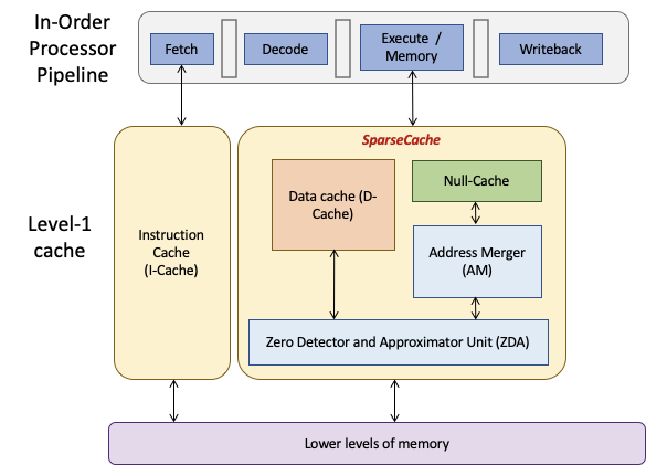
Features
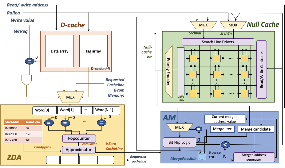
- A TCAM based write-through null-cache to store zero-cache line addresses
- A Zero Detector and Approximator to detect zero-cache lines and approximate near zero-cache lines (Challenge 1)
- An Address Merger to find and merge contiguous and strided cache lines (Challenge 3)
- An augmented replacement policy for null-cache to preferentially retain zero cache-lines
Solution: SparseCache
Experimental Methodology
-
SparseCache was integrated into a low-end Intel processor (configuration similar to Intel Galileo boards) and evaluated using an in-house developed x86 simulator based on Intel’s pin-tool
-
Four pruned image-recognition DNNs used as benchmarks
0.1% area and 3.8% power overhead
[1]. Yu et. al, Scalpel: Customizing DNN pruning to the underlying parallelism , ISCA 2017
[2]. Han et. al, Deep Compression: Compressing DNNs with Pruning, Trained Quantization and Huffmann Encoding, ICLR 2016
| Processor Config. | Intel Atom, in-order |
|---|---|
| Operating Freq. | 400 MHz |
| L1 Data Cache | 16 KB, 4 way SA, 32B/Block, 1 cycle hit latency |
| Null-Cache | 1KB, address only, TCAM, 1 cycle hit latency |
| Main Memory Cycles | 100 cycles |
| Benchmarks | Pruning | Dataset | No. layers |
|---|---|---|---|
| LeNet | Scalpel [1] | MNIST | 5 |
| AlexNet | DC [2] | ImageNet | 8 |
| VGG-16 | DC [2] | ImageNet | 16 |
| SqueezeNet | DC [2] | ImageNet | 26 |
Results: Performance improvements
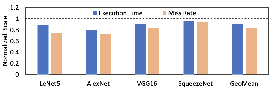
- 5-21% reduction in application execution times across all benchmarks
- 5-28% reduction in cache miss-rates across all benchmarks
- Benefits proportional to number of zero-valued cache lines
- Miss rate reductions will lead to system-wide energy benefits due to reductions in off-chip memory accesses
Results: Performance improvements of SparseCache (16KB+1KB) over bigger Data-Cache (32KB)

- A 16KB data-cache + 1KB null-cache is as performant as a significantly higher area and power consuming 32KB data-cache
-
Additionally, SparseCache configuration gives 13% and 20% benefits in execution time and miss rates respectively on AlexNet
Summary
- We propose SparseCache, light-weight cache extensions to general purpose processors to speed up DNN execution by exploiting sparsity
- SparseCache consists of a TCAM based null-cache, ZDA and AM to detect and store zero valued addresses compactly
-
Light-weight extensions to GPPs are a viable alternative to custom hardware design, for resource-constrained devices
-
Results
-
5-21% application execution time reduction across 4 benchmarks
-
Same or better performance than a 2X larger data-cache with less than half its size
-
Our thesis
Efficient Deep Learning
Efficient Systems
SparseCache
Efficient Design Methodology
Generalizable cost models
Efficient Neural Networks
FuSeConv
Our thesis
Efficient Deep Learning
Efficient Systems
SparseCache
Efficient Design Methodology
Generalizable cost models
Efficient Neural Networks
FuSeConv
IISWC 2020
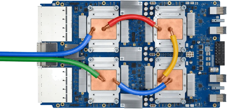
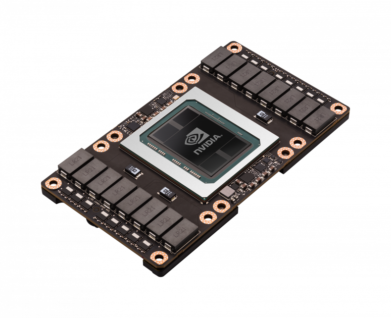
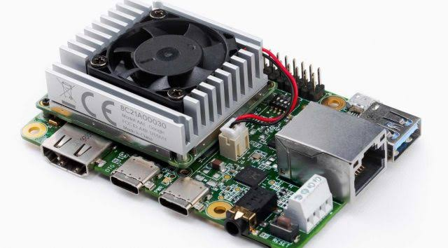
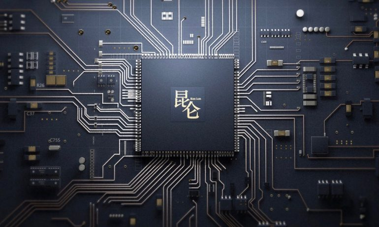

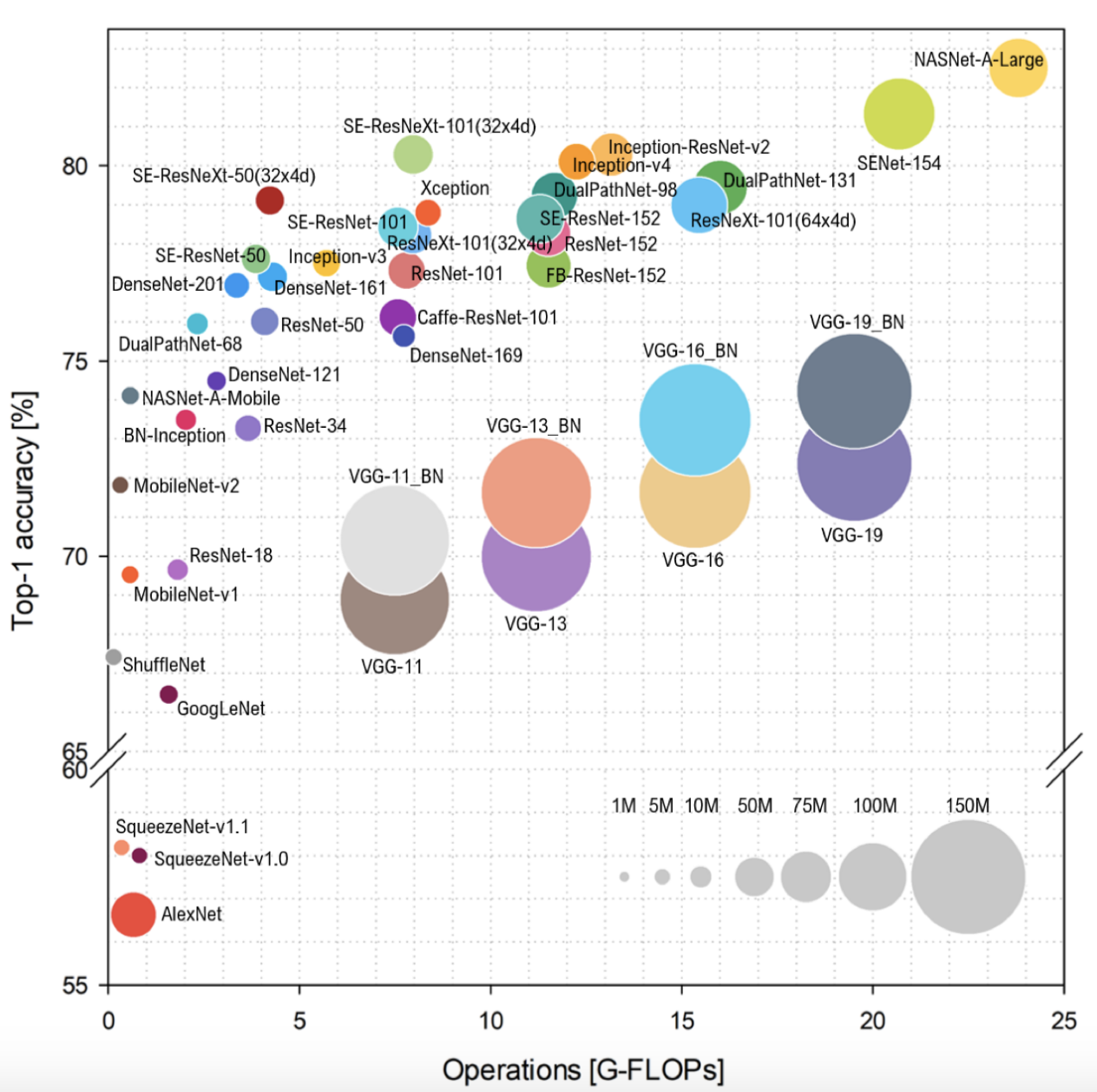
Characterizing each DNN on each hardware is infeasible
Source: Reddi et.al, MLPerf Inference Benchmark, ISCA 2020
Motivation: Exploding product space of DNNs and devices
Insight: Build Cost Models to Estimate Latency


N times
Latency

DNN Representation
Trained with many DNN, latency pairs to generalize to unseen DNNs
Learn an ML model that can predict the latency of a network on a device
How do we generalize this to multiple hardware devices?


DNN Representation
HW Representation
Latency
Key idea: A unique hardware representation for the cost model
Solution: Generalizable Cost Models
Challenges
- Collecting a large dataset across networks and devices
- Uniquely representing a hardware
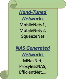


Android App
Central Database
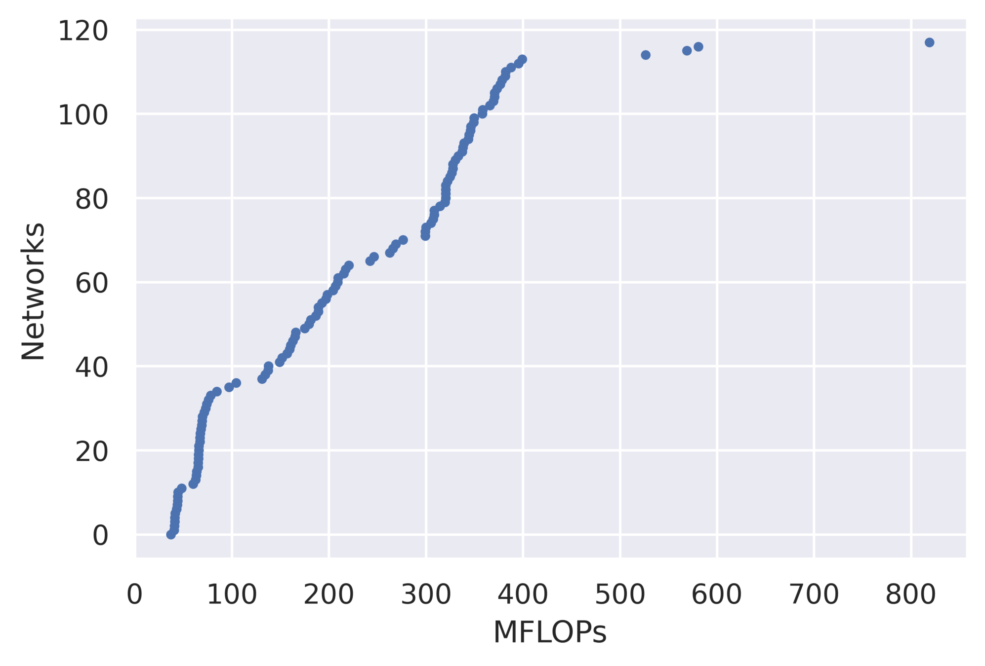
118 networks
105 mobile devices
Challenge: Collecting a large dataset
Challenge: Collecting a large dataset
Visualizing the Data
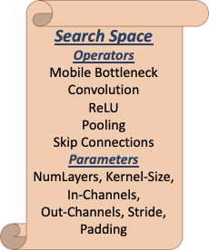
A diverse set of DNNs ranging from 40-800 MFLOPs spanning across many operators and parameters
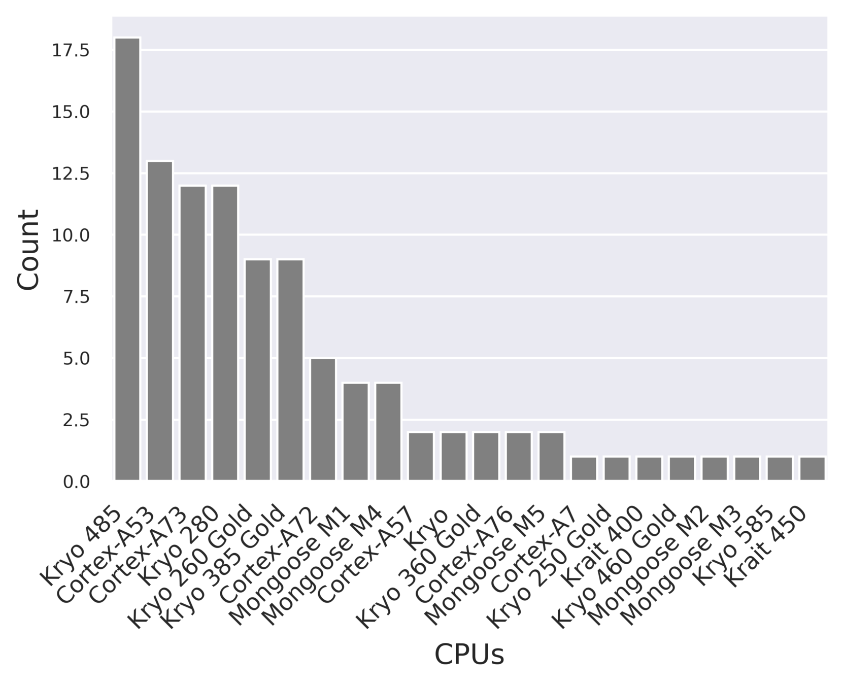
Significant diversity in devices ranging from an 8-year old Cortex-A53 to 9 month old Kryo 585


DNN Representation
Latency
Challenge: Uniquely representing a hardware
Challenges
- Collecting a large dataset across networks and devices
- Uniquely representing a hardware
Can we use simple features such as core freq, DRAM size, etc.
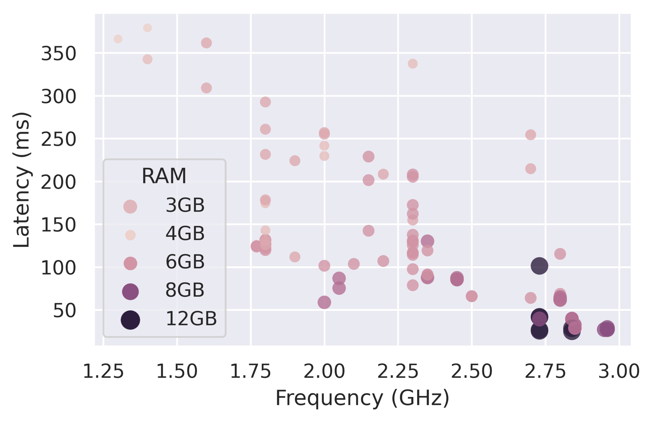
2.5x latency variability for the same frequency and DRAM size
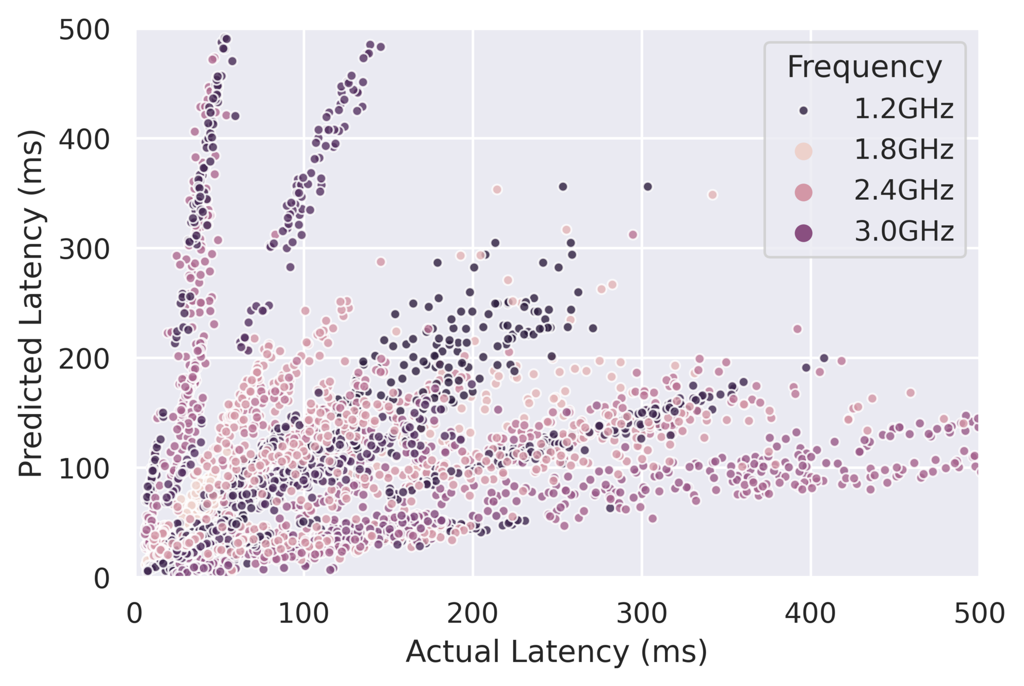
Poor predictive power for a cost model learnt with frequency and DRAM size
Using static hardware features (CPU Freq, DRAM size, etc.) as the representation
Do simple features work?


DNN Representation
Latency



100.4
350.55
59.6
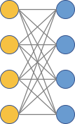
Unique fingerprint for a hardware
Key Question: How to choose the DNNs for the Signature Set?
Solution: Signature Set Representation
Represent a device by its latency on a set of DNNs - the signature set
We propose three methods to select the signature set from the set of 118 networks.
- Random Sampling (RS)
- Mutual Information based Sampling (MIS)
- Spearman Correlation Coefficient based Sampling (SCCS)
Solution: Selecting Signature Sets
We are interested in DNNs that help discriminate the hardware devices.


XGBoost
\( R^2 \): Coefficient of Determination
70% of devices as the training set, 30% as the test set
Only training set participates in signature set selection
Experimental Methodology
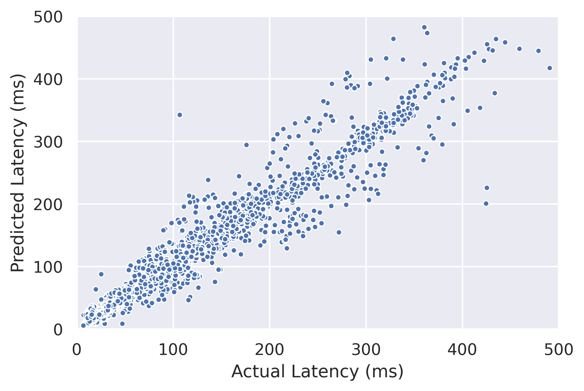
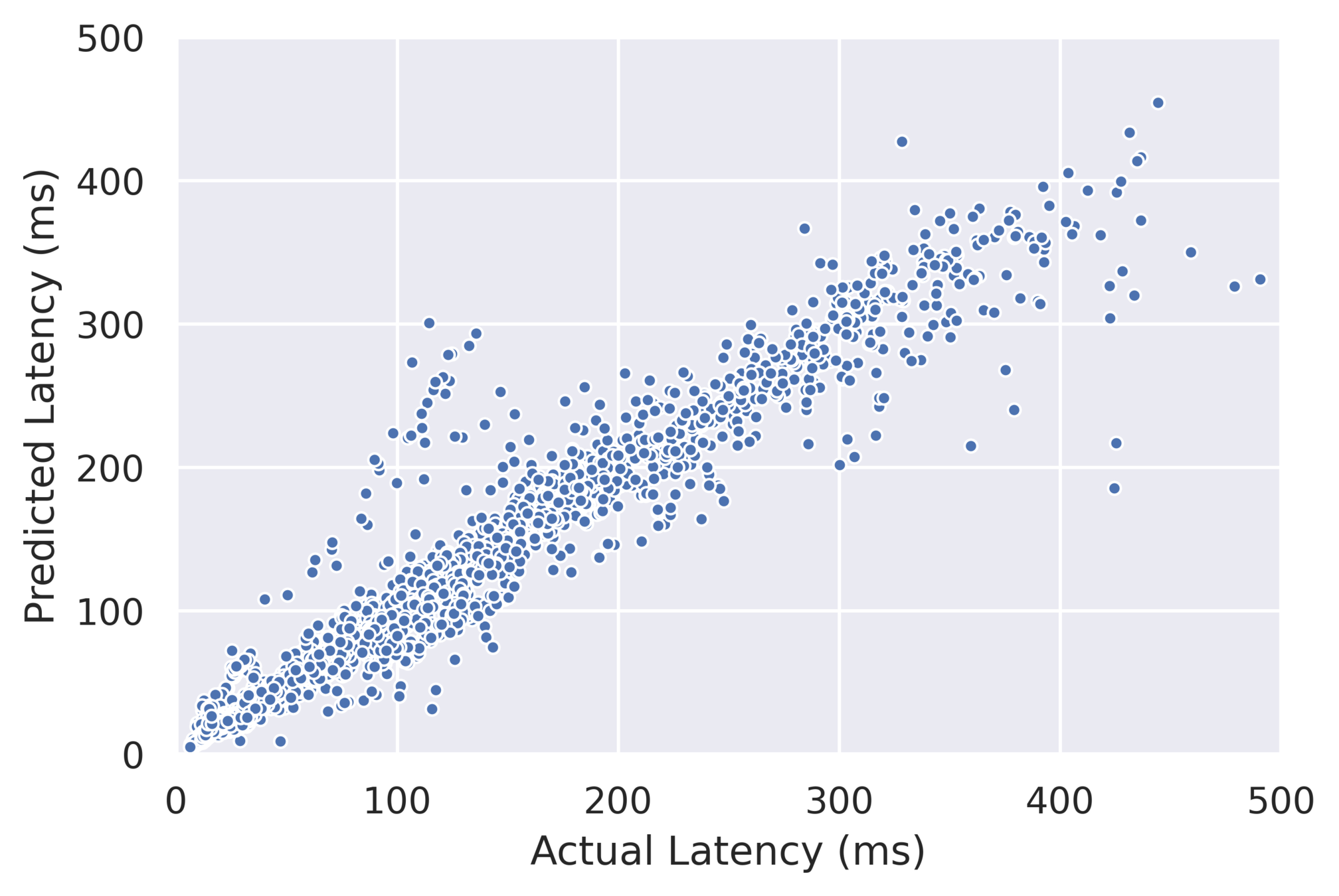
Results: Performance of Cost Models
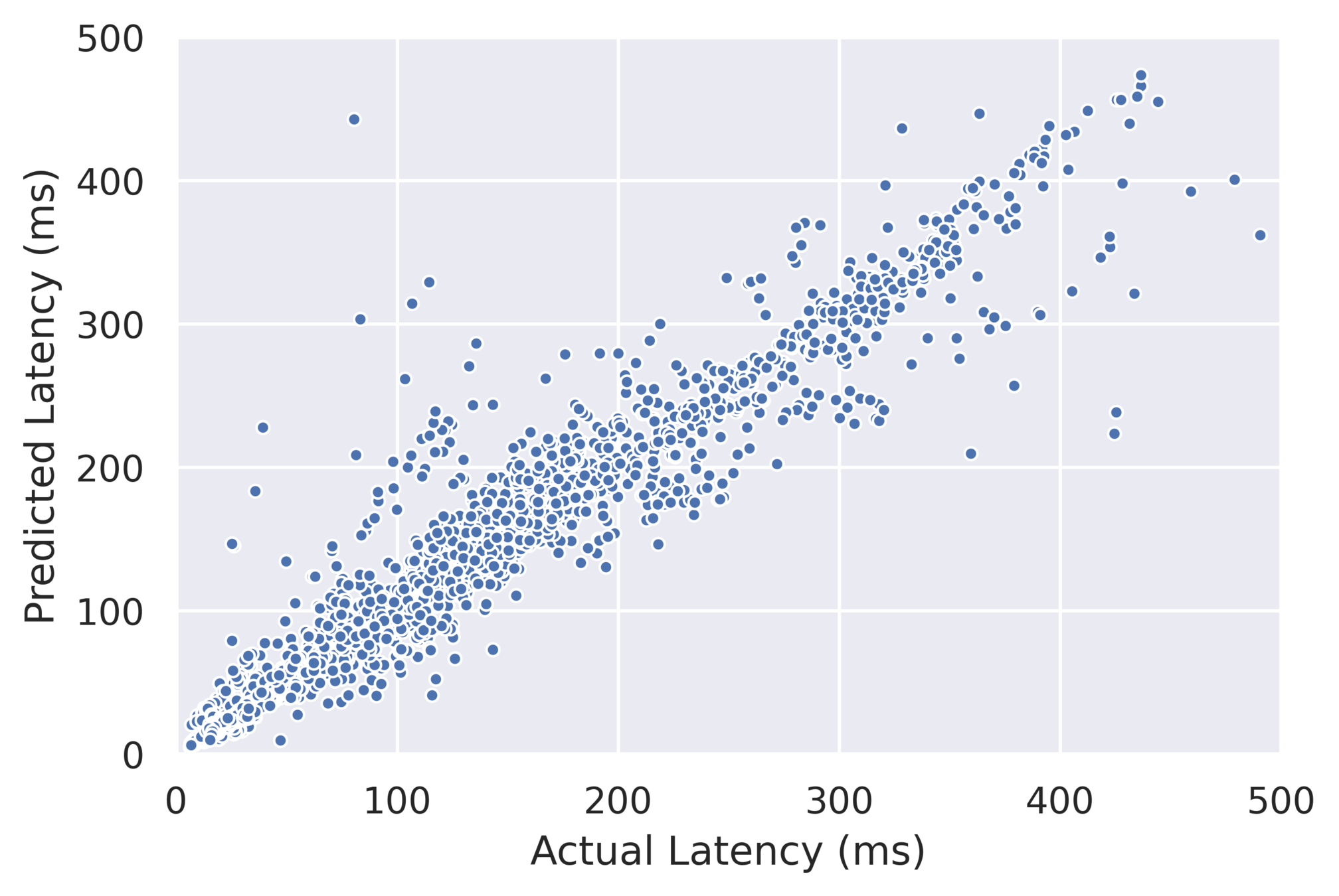
RS: \( R^2 \) = 0.9125
SCCS: \( R^2 \) = 0.944
MIS: \( R^2 \) = 0.943
The cost model generalizes well to unseen mobile devices
Interesting Questions:
- Does Random Sampling always perform well?
- What is the optimal number of networks in the signature set?
Results: Consistency of Random Sampling
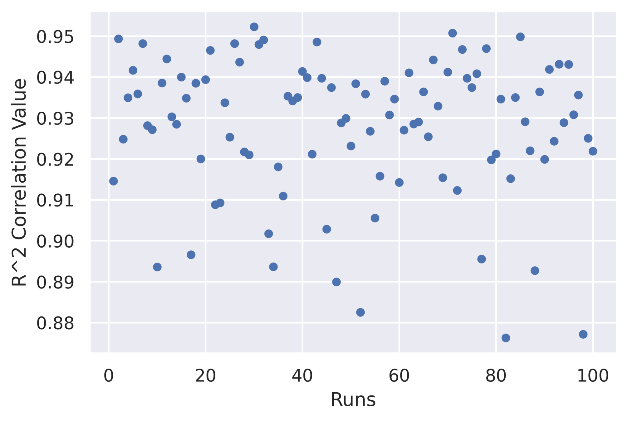
- Performs competitively well on average
- Outliers perform poorly
Mean \( R^2 \) = 0.927
MIS, SCCS
Results: Optimal number of networks in Signature Set
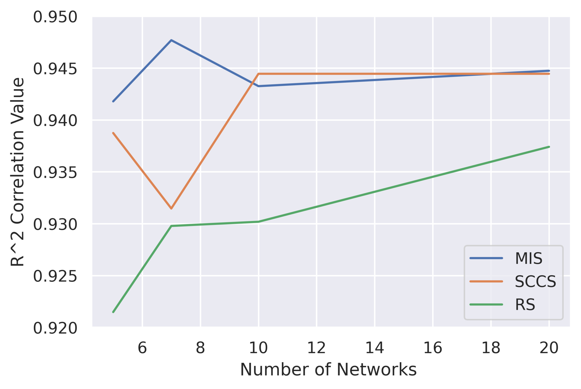
- Ideal size: 5-10 networks (4-8% of all networks)
- Very small signature set to effectively describe a hardware

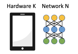

Predicted: 70 ms
Actual: 25 ms

Learning


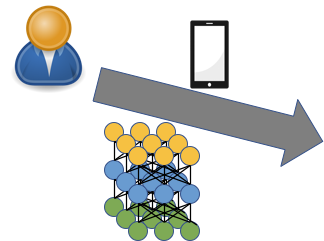
Inference
Predicted: 24.5 ms
Actual: 25 ms
Application in practice: Collaborative Workload Characterisation
Results: Simulation with 50 devices in collaboration
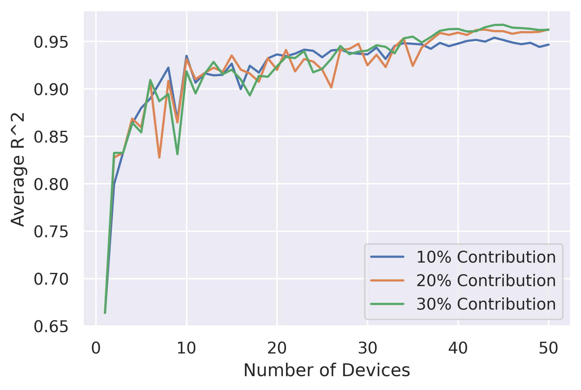
Even for 10% contribution from each device, the model shows superior \( R^2 \) values
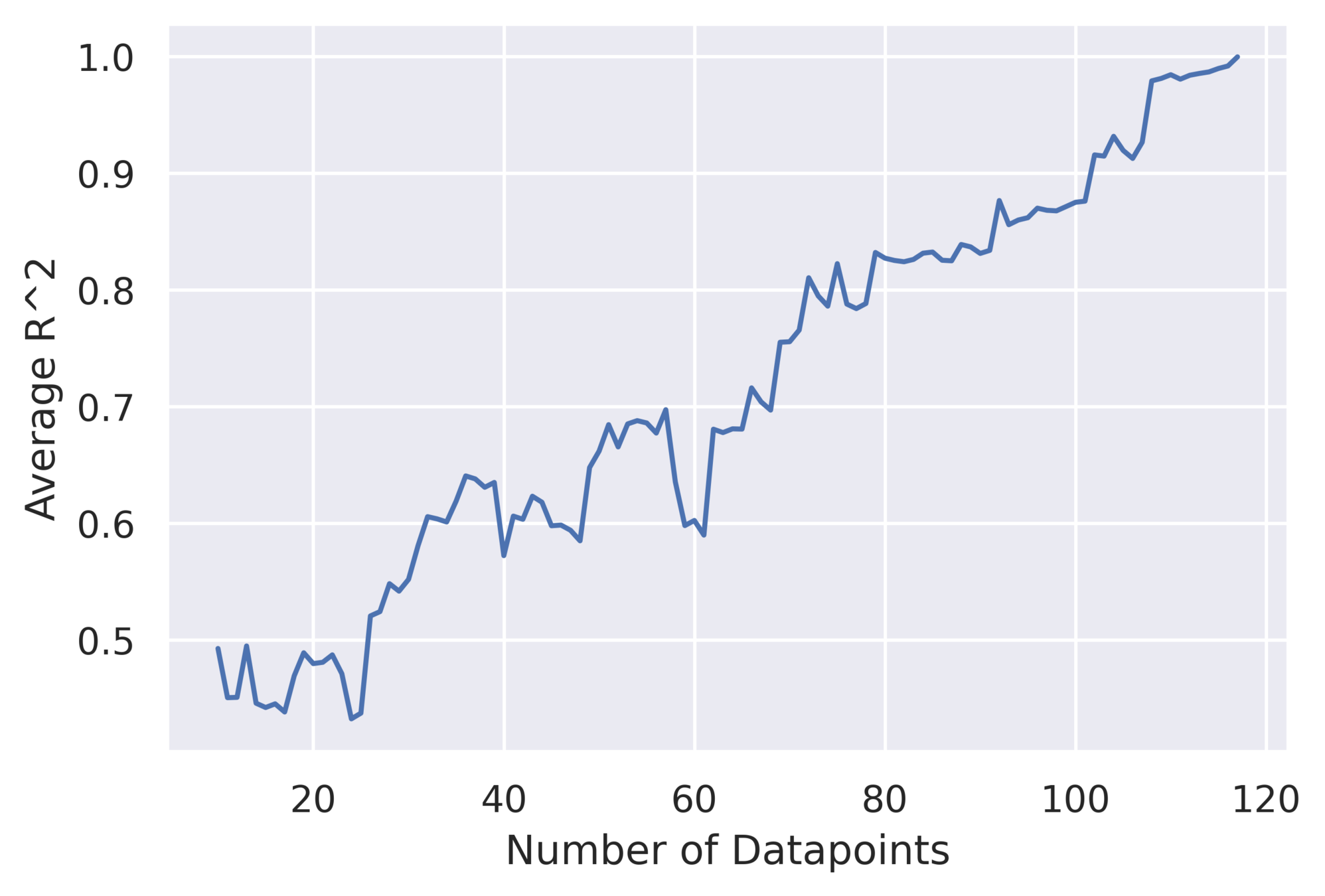
11x
Collaborative \( R^2 \): 0.98
11x lower characterisation cost for collaborative model compared to the unique model
Extremely small contributions from many people \( \implies \) accurate generalizable cost models
Summary
- Characterizing latency of DNNs on hardware devices is challenging due to network and hardware diversity
- We need accurate cost models to effectively characterize networks on devices
- We proposed a superior cost model that generalizes across both networks and mobile devices on a real-world dataset
- The model utilizes a novel and easy-to-obtain representation of devices using latencies on a signature set of DNNs
- We showed a practical setting of building such a generalizable cost model in a collaborative manner
- We believe such a cost model will significantly reduce the computational and environmental overhead in characterizing DNNs on devices
Our thesis
Efficient Deep Learning
Efficient Systems
SparseCache
Efficient Design Methodology
Generalizable cost models
Efficient Networks
FuSeConv
Our thesis
Efficient Deep Learning
Efficient Systems
SparseCache
Efficient Design Methodology
Generalizable cost models
Efficient Networks
FuSeConv
DATE 2021
Motivation: Accelerators and Efficient Operators
Systolic-arrays and depth-wise separable convolutions are ubiquitous for efficient inference
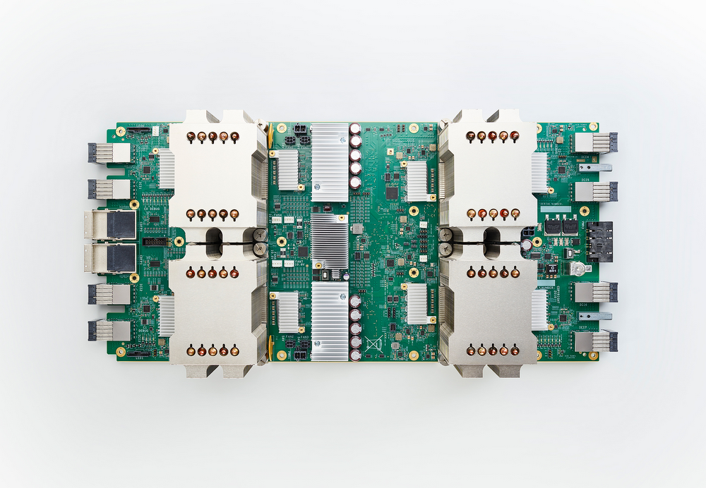
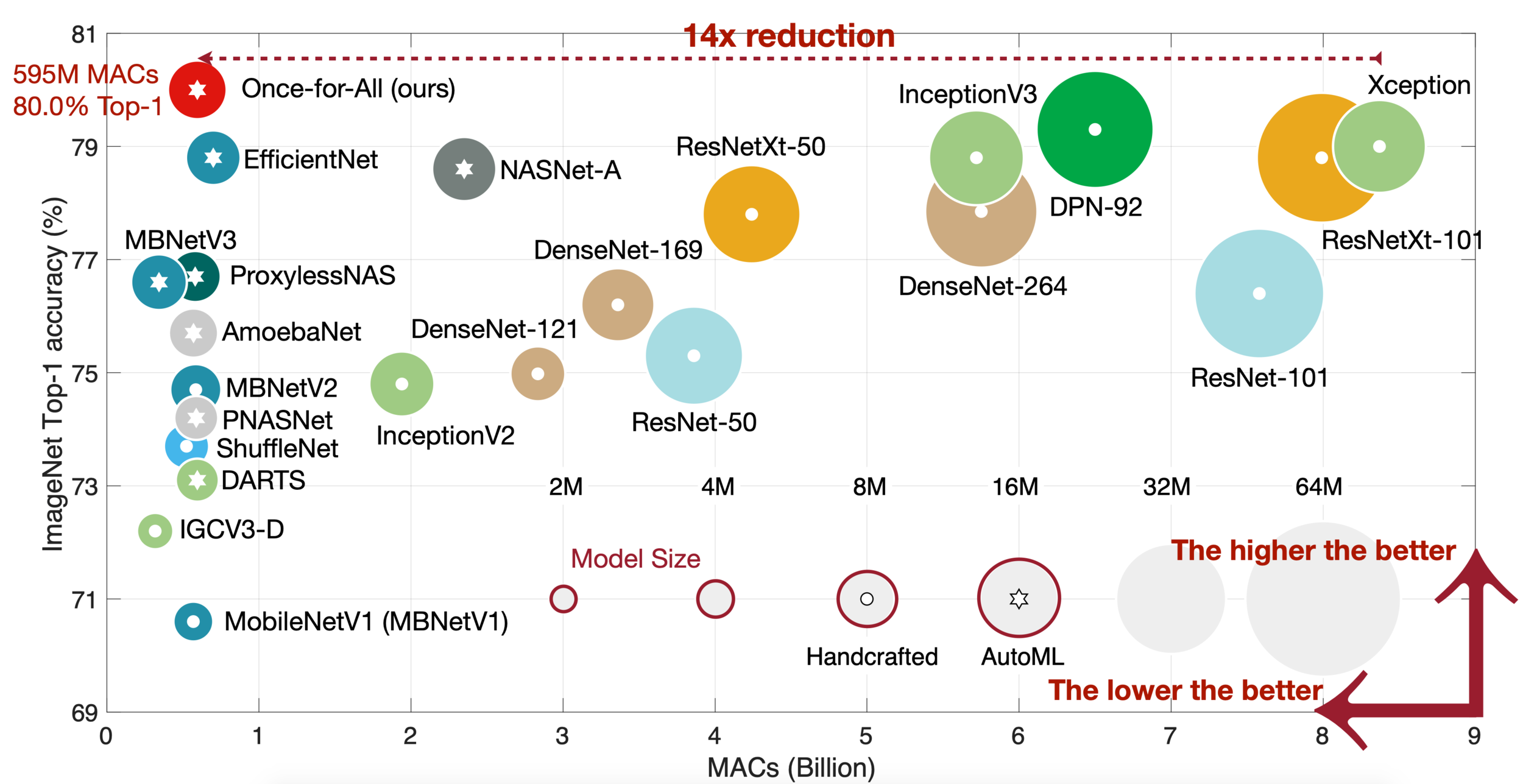
25-29x more performant over GPUs
12/12 efficient networks use depth-wise separable convolutions
Source: Han Cai et. al, Once For All, ICLR 2019
Source: TPU, cloud.google.com
Motivation: The combination of both is inefficient
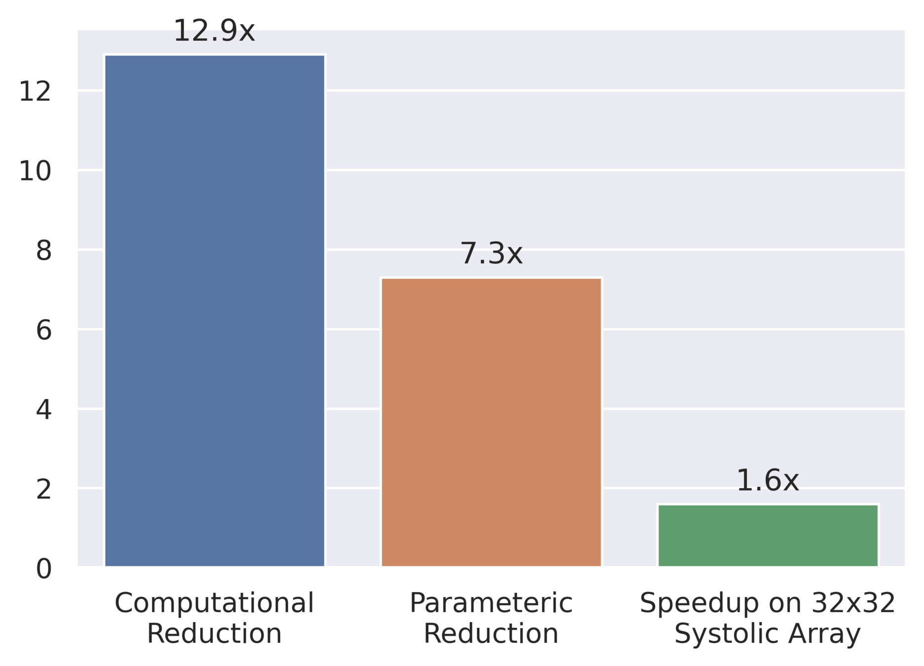
Comparing MobileNet-V2 with ResNet-50
Incommensurate
Scaling
> Why are Depth-Wise (DW) convolutions inefficient on systolic arrays?
> What can we do to make DW convolution faster on systolic arrays?
> How good is the inference performance of our proposed solution?
Background
Standard Convolution
Depthwise Separable Convolution = Depthwise Conv + Pointwise Conv
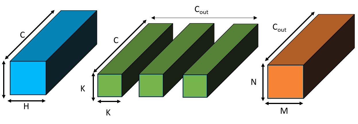

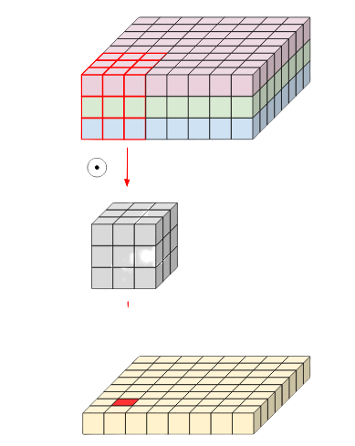
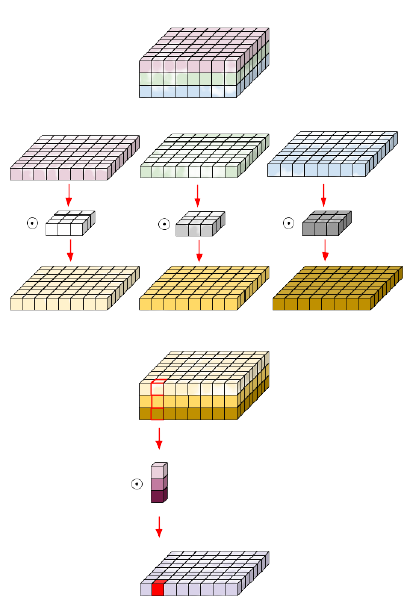
\( (N \times M \times C \times K^2 \times C_{out}) \)
\( (N \times M \times C \times (K^2 + C_{out})) \)
Upto \( K^2 \) times reduction in computations
Insight: Depth-wise convolutions poorly utilize systolic-arrays
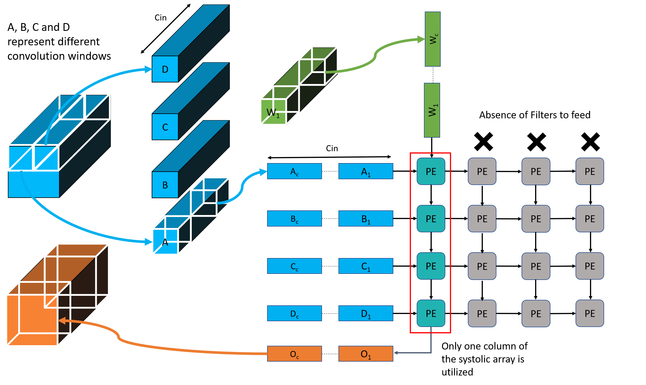
Solution: FuSeConv


Fully Separable Convolution (FuSeConv) : Composes of 1D depthwise convolutions and pointwise convolution
Depthwise Separable Convolution
Full Variant (D = 1)
Half Variant (D = 2)
Solution: FuSeConv
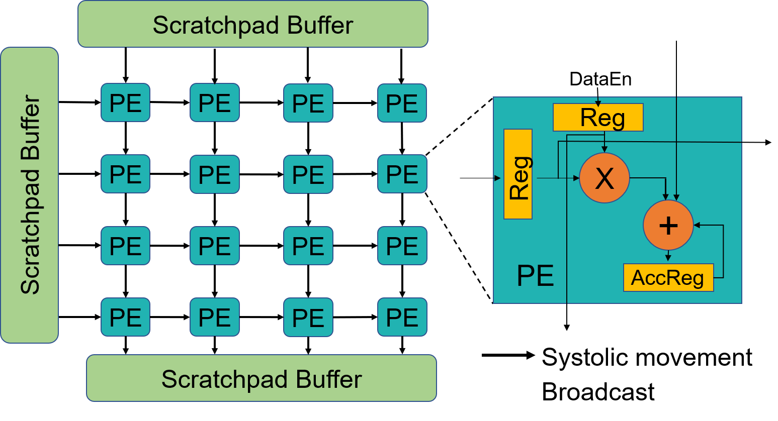
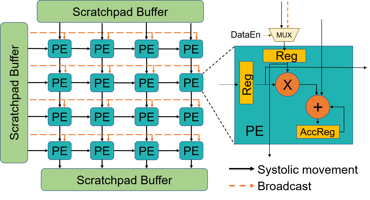
Execute independent 1D convolutions
On 32 x 32 array
| Area | 4.35% |
| Power | 2.25% |
Solution: FuSeConv Mapping
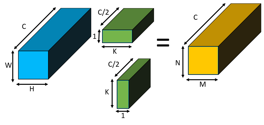

All PEs are completely utilized due to the 1D convolutions of FuSeConv and modified dataflow
Experimental Methodology
> Evaluate 4 FuSe variants and compare with baseline
> Latency simulator based on SCALE-SIM [1] from ARM and Georgia Tech
> MobileNets (V1, V2, V3-Small, V3-Large) and MnasNet-B1
Choose half of layers greedily to maximize speedup of layer
> Full (D = 1) FuSe
> Half (D = 2) FuSe
> 50% Full FuSe
> 50% Half FuSe
All layers are replaced with FuSeConv
[1]. Samajdar et. al, SCALE-Sim: Systolic CNN Accelerator Simulator, ISPASS 2020
Results
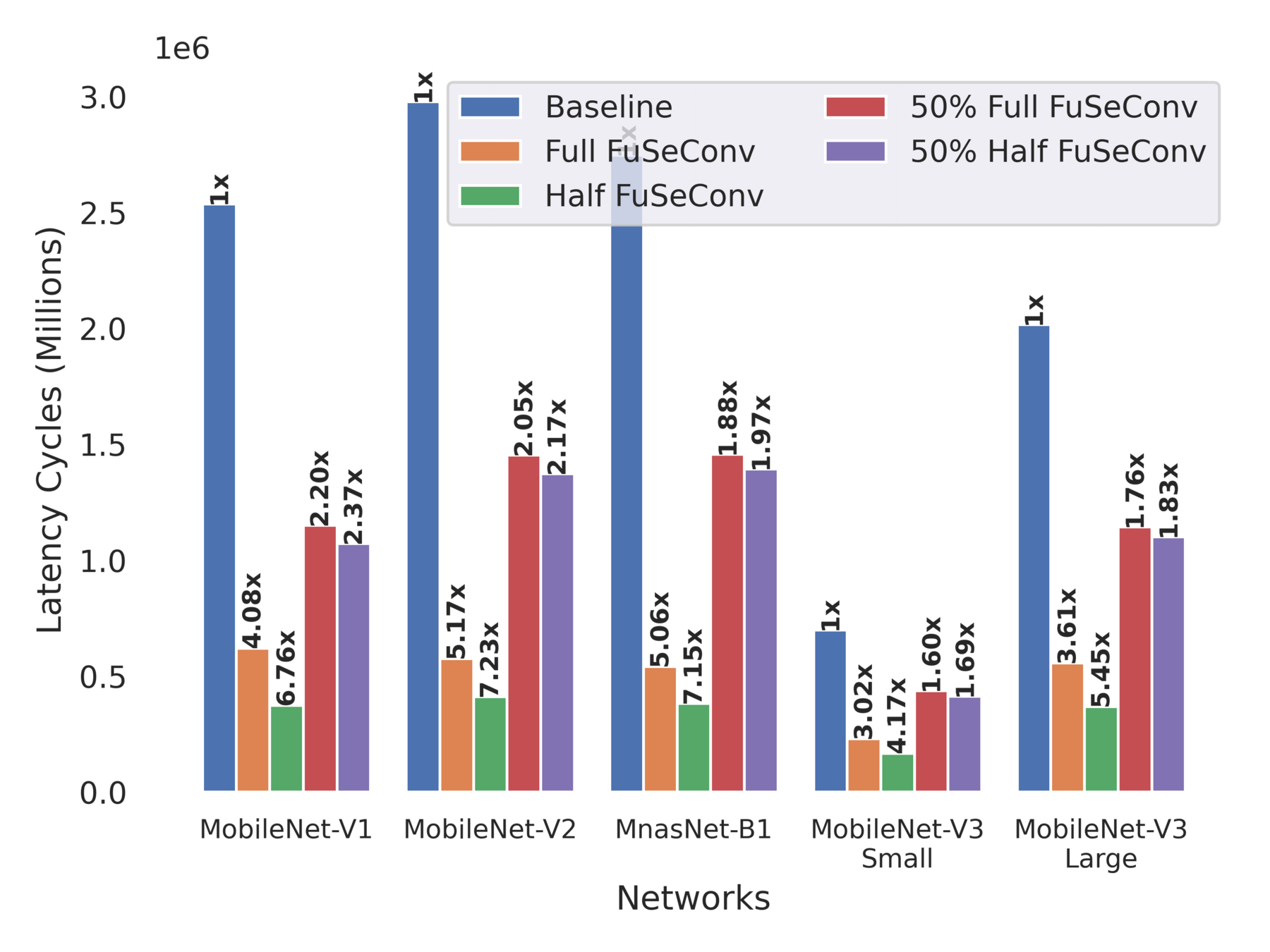
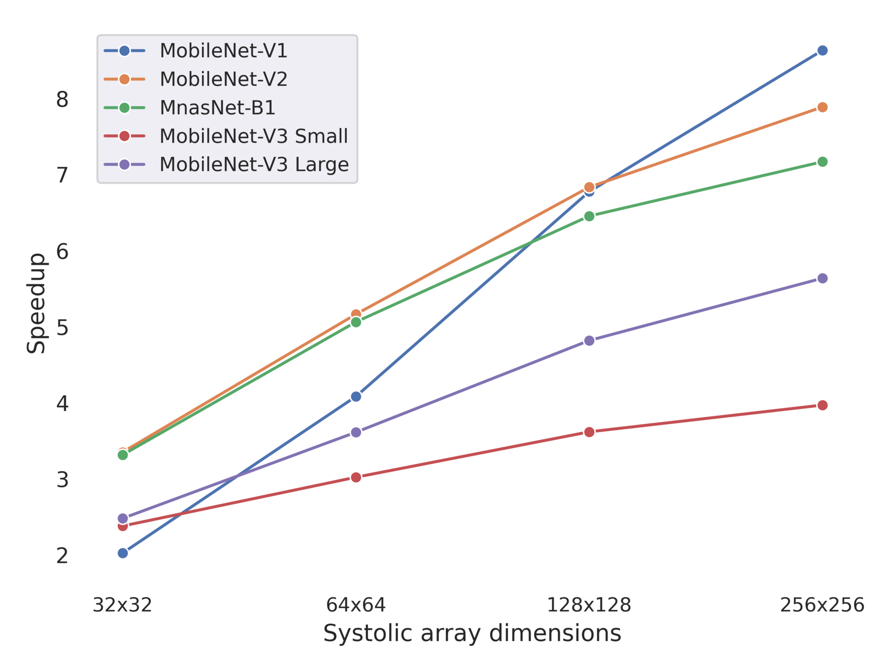
Average accuracy drop of ~1% in Half variants, and ~0.3% in Full variants
Upto 7.23x improvements in execution time
Summary
- Widespread solutions for efficient inference are Hardware Accelerators and Efficient DNN Operator
- However, Depthwise Separable Convolutions are inefficient on Systolic Arrays and lacks data reuse to exploit parallelism
- We propose FuSeConv (Fully Separable 1D Convolutions) as a drop-in replacement for Depthwise Separable Convolutions
- To improve the utilization, we also proposed a modified dataflow for systolic-arrays
- Our solution is atleast 3-7X faster than efficient mobile networks such as MobileNets and MnasNet with negligible accuracy-drop
Conclusion
Efficient Deep Learning
Efficient Systems
SparseCache
Efficient Design Methodology
Generalizable cost models
Efficient Neural Networks
FuSeConv


Future Work
Efficient DNN Training

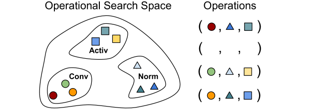
Efficient Operators
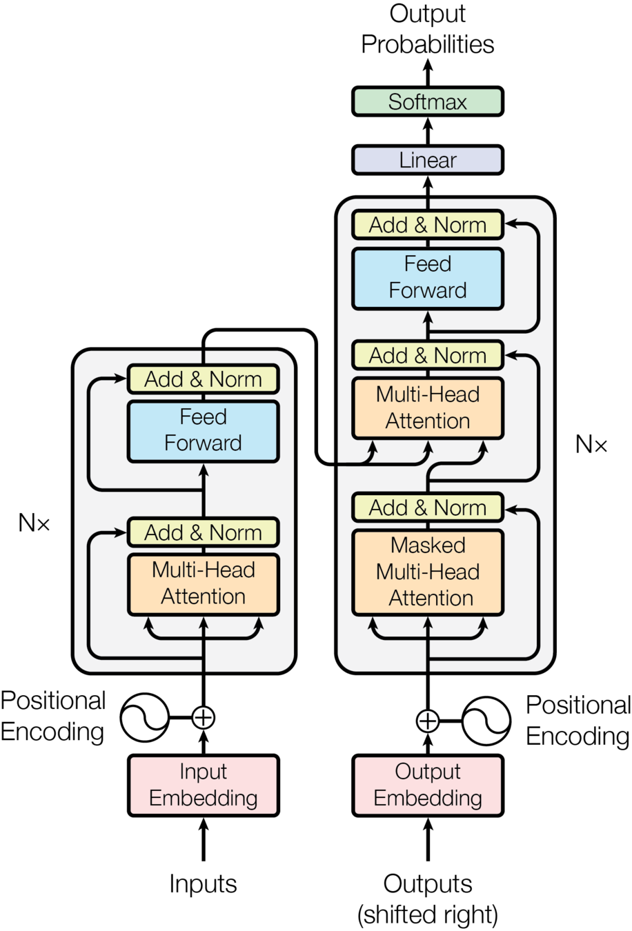
Efficient Transformers
Thank You
Questions?
Backup Slides


Fast devices with 50ms mean latency
Medium fast devices with 115ms mean latency
Slow devices with 235ms mean latency
A mobile device with latency distribution of 118 networks
Visualizing the Data
Systolic Algorithms
> A class of algorithms that runs efficiently on systolic architectures
> Computational loops are transformed into Regular Iterative Algorithm (RIA)
> RIAs that have constant offsets only can be synthesized on systolic arrays


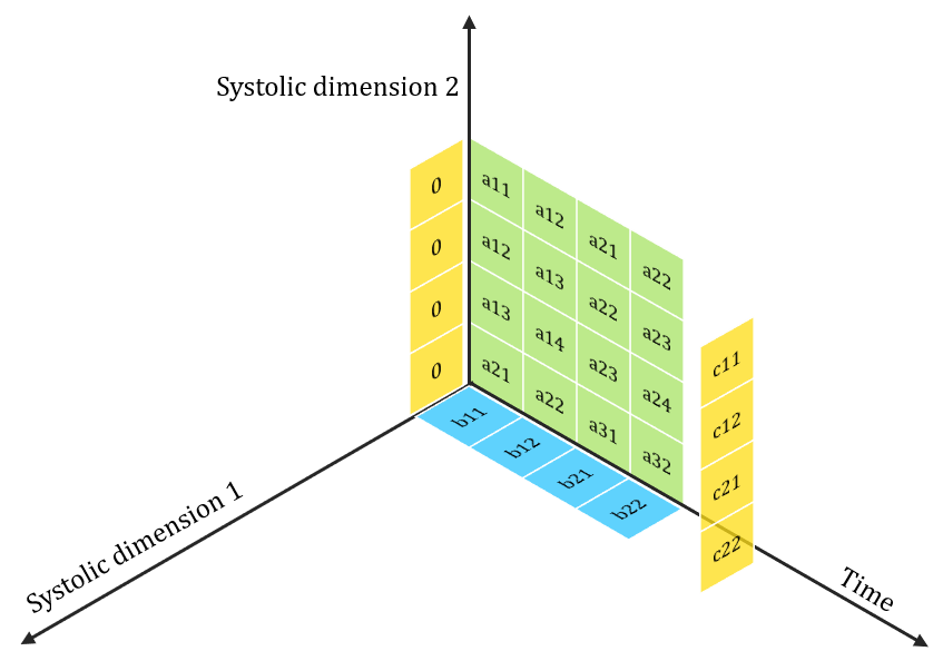
Mapping Systolic Algorithms to Systolic Arrays
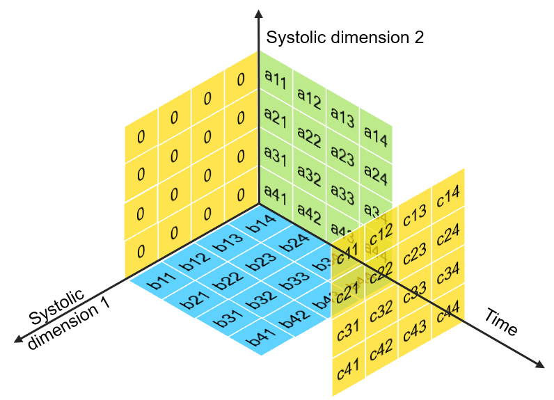
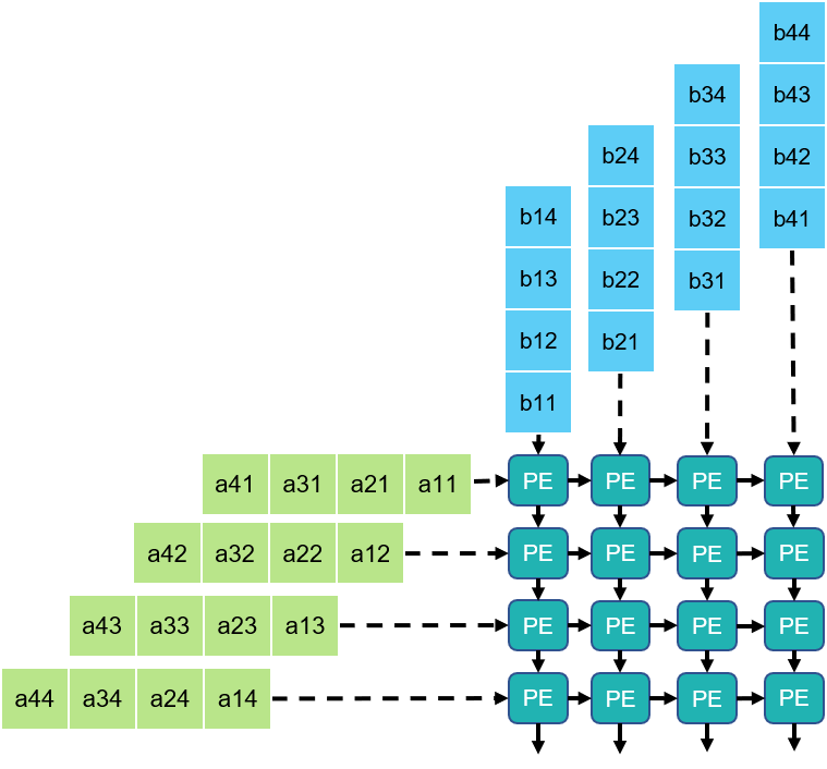


> i, j indices maps to Spatial dimensions of array
> k index maps to Temporal dimension
Time
Dim1
Dim2
What about 2D Convolutions?


> Non-Constant Offset indices in RIA


> 2D Convolution is not a Systolic Algorithm
Then how are 2D Convolutions mapped onto Systolic Arrays?


After im2col transformation
Under Utilization
Then, How to make them efficient on Systolic?
> More filters -> Data reuse -> High Utilization
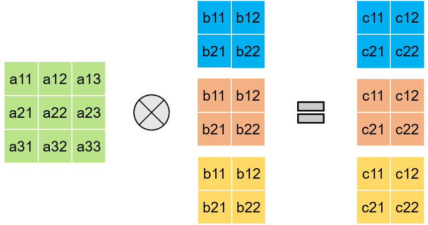
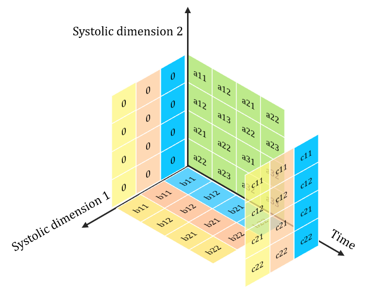
> Extendable for convolution with channels too
2D Convolution with Multiple Filters
FuSeConv is a systolic algorithm !
> FuSeConv composes of only 1D convolutions.

> 1 x K & K x 1depthwise convolutions
> 1 x 1 Pointwise Convolution
Matrix Multiplication
1D Convolutions


> Constant Offset => Systolic Algorithm
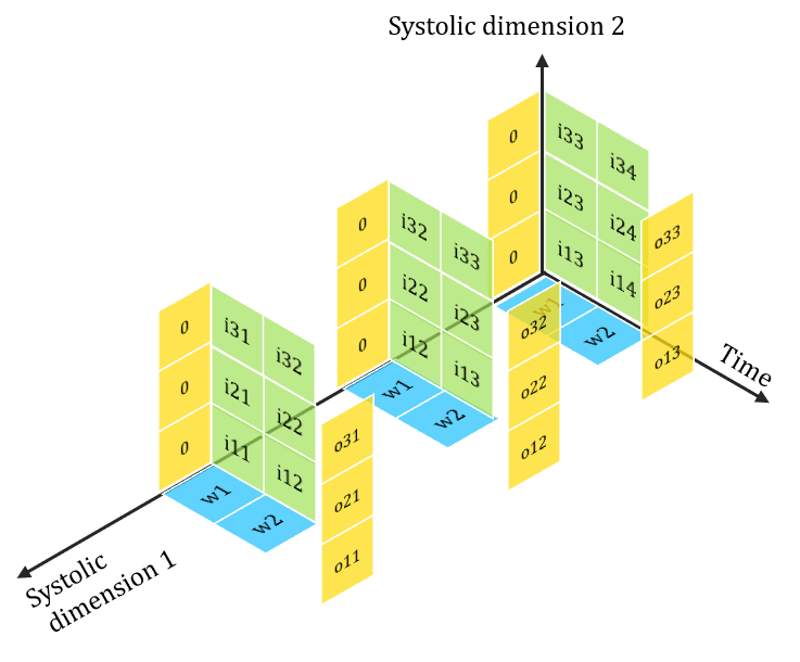
Efficiency of FuSeConv on our Proposed Hardware


Channel 0
Channel 1
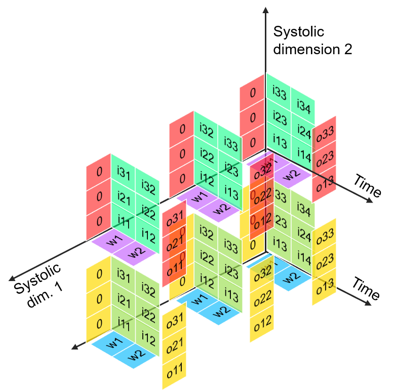
> Channelwise 1D convolutions can be computed in parallel
> FuSeConv + our dataflow mapping exploits parallelism which were absent in depthwise convolutions mapping natively on Systolic Arrays
Multiple Channels can execute in parallel along dimension 2
Evaluation
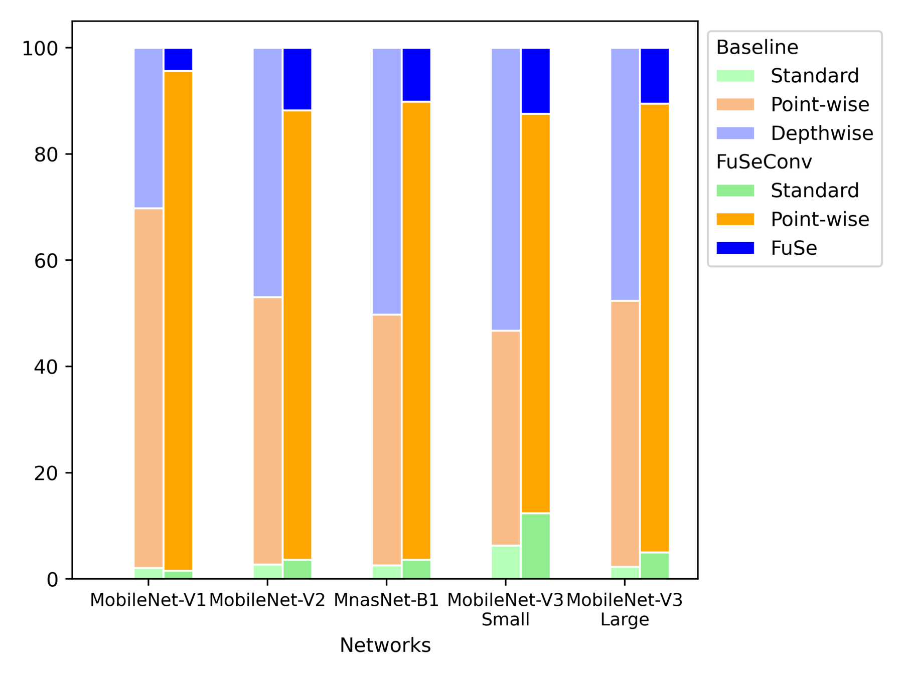
Operator-wise Latency Distribution of Full FuSe Variants
Layerwise Speedup of MobileNet-V2 Full FuSe Variant
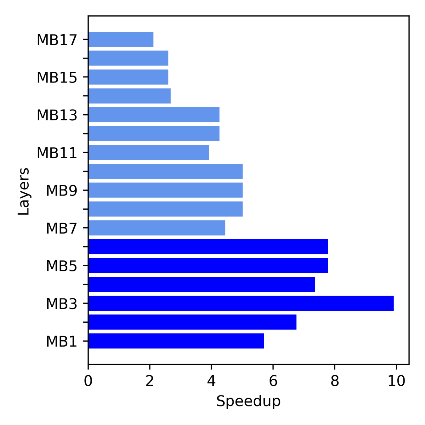
More Speedup from Initial layers
Inference latency dominated by Depthwise -> Point-wise