Repeated-Measures ANOVA

Vít Gabrhel

vit.gabrhel@mail.muni.cz

FSS MU,

14. 11. 2016

Repeated Measures

Repeated Measures ANOVA

Úvod

• Slouží pro srovnání skupinových průměrů napříč 3 a více podmínkami 
• Within-subject a longitudinální design:
  • Sledujeme vývoj nějaké proměnné v čase 
  • Vystavujeme stejné jedince několika experimentálním podmínkám a hledáme rozdíl ve změně 

Představuje řešení situace, kdy je při opakovaných měřeních porušen předpoklad ANOVA či lineární regrese o nezávislosti pozorování

Repeated Measures ANOVA

Rozptyl v rámci Repeated Measures ANOVA (dle Field, 2012)

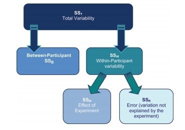
Repeated Measures ANOVA

Rozptyl v rámci Repeated Measures ANOVA (dle Field, 2012)

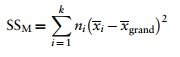
 Variabilita mezi měřeními (SSM)

 We worked out how much variation could be explained by our experiment (the model SS) by looking  at the means for each group and comparing these to the overall mean. So, we measured the  variance resulting from the differences between group means and the overall mean

1. Calculate the difference between the mean of each group and the grand mean.
2. Square each of these differences.
3. Multiply each result by the number of participants that contribute to that mean (ni ).
4. Add the values for each group together:

 Variabilita mezi subjekty (SSW)

 This equation simply means that we are looking at the variation in an individual’s scores and  then adding these variances for all the people in the study. The ns simply represent the number  of scores on which the variances are based

• Variance created by individuals' performances under different conditions
  • Some of this variation is the result of our experimental manipulation and some of this variation is simply random fluctuation.

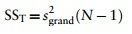
 Celkový rozptyl (SST)

• The grand variance in the equation is simply the variance of all scores when we ignore the group to which they belong

Repeated Measures ANOVA

Rozptyl v rámci Repeated Measures ANOVA (dle Field, 2012)

 

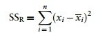
Chybový rozptyl (SSR)

• The final sum of squares is the residual sum of squares (SSR), which tells us how much of the variation cannot be explained by the model.
  • This value is the amount of variation caused by extraneous factors outside of experimental control

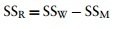
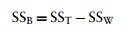
The between-participant sum of squares (SSB)

• This term represents individual differences between cases
  • Its value is the amount of variation caused by differences between individuals

Repeated Measures ANOVA

Rozptyl v rámci Repeated Measures ANOVA (dle Field, 2012)

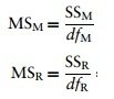
The mean squares

SSM tells us how much variation the model (e.g. the experimental manipulation) explains and SSR tells us how much variation is due to extraneous factors.

• However, because both of these values are summed values the number of scores that were summed influences them. We eliminate this bias by calculating the average sum of squares.

F-ratio

• The F-ratio is a measure of the ratio of the variation explained by the model and the variation explained by unsystematic factors.

  • It can be calculated by dividing the model mean squares by the residual mean squares

Repeated Measures ANOVA

Rozptyl v rámci Repeated Measures ANOVA

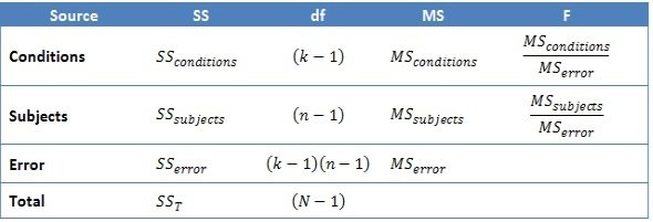
k - počet podmínek (treatments)

n - počet participantů (pozorování)

df_Total - number of observations (across all levels of the within-subjects factor, n) – 1

Repeated Measures ANOVA

Výhody

​Vyšší statistická síla 

• ​The repeated measures design is statistically more powerful because of the change in the nature of the error term or the unsystematic variance. Subjects may consistently reveal individual differences.
  • For example: participants which are not taking the experiment seriously, do not gain anything in the working memory training. So, they will not show an effect.
• Repeated measures design will take this variability across subjects into account and will see whether there is systematic variability that can be contributed to the individual people.

 

​Menší počet potřebných participantů

• Nižší náklady (je třeba méně zkoumaných osob)

Repeated Measures ANOVA

Nevýhody

Order effect

• Jak ošetřit vliv pořadí experimentálních podmínek na sledovanou proměnnou?
  • Counterbalancing
    • Randomised -  A2,A1,A1,A2
      • Randomizace pořadí podmínek
    • Blocked - a) A1,A2 b) A2,A1
      • Náhodné zařazení do skupiny reprezentující pořadí podmínek
  • Latin Square - Každý respondent je vystaven každému pořadí experimentálních podmínek právě jednou

Missing values

• Vzhledem k obvykle menšímu počtu participantů představuje riziko - změnou variability či výpočetní komplikací (kupř. fit modelu)
  • Otázka nakládání s chybějícími daty - listwise, pairwise, vážení atd.
  • Souvisí s povahou chybějících dat - MCAR, MAR, MNAR

Repeated Measures ANOVA

Data: Cognitive training

• Four independent groups (8, 12, 17, 19 sessions)
• Measured IQ of 20 subjects after 4 sessions of training
• Dependent variable is IQ gain after a particular session
• Null hypothesis: There are no differences among the treatment groups
• Alternative hypothesis: There is one (or more) mean differences among the treatment groups

Repeated Measures ANOVA

Data: Cognitive training

setwd()
dir()

 

install.packages("readxl")
library("readxl")

 

excel_sheets("RMANOVA.xlsx")

RMANOVA = read_excel("RMANOVA.xlsx", sheet = 1)
View(RMANOVA)

 

RMANOVA$condition2 = factor(RMANOVA$condition, order = TRUE, levels = c("8 days", "12 days", "17 days", "19 days"))

RMANOVA$subject2 = factor(RMANOVA$subject, order = FALSE)

Repeated Measures ANOVA

Statistický popis dat

 # Summary statistics by group

 library(psych)
 describeBy(RMANOVA, group = RMANOVA$condition2)

 

# Boxplot

 library(ggplot2)
 bp1 = ggplot(RMANOVA, aes(condition2, iq))

 bp1 + geom_boxplot(aes(fill=condition2), alpha=I(0.5)) +
  geom_point(position="jitter", alpha=0.5) +
  geom_boxplot(outlier.size=0, alpha=0.5) +
  theme(
    axis.title.x = element_text(face="bold", color="black", size=12),
    axis.title.y = element_text(face="bold", color="black", size=12),
    plot.title = element_text(face="bold", color = "black", size=12)) +
  labs(x="Condition",
       y = "IQ gain",
       title= "IQ gain by the days of training") + theme(legend.position='none')

Repeated Measures ANOVA

F-test a F-Ratio

Funkce aov

• Because you're using repeated measures, you have to add a term Error(wm$subject / wm$condition).
  • This term tells R that you need a special error term since you are working in a repeated measures design and the error term differs.
• So you add this term, saying that the subjects are measured repeatedly across conditions.

 

 # Apply the aov function

model <- aov(iq ~ condition2 + Error(subject2 / condition2), data = RMANOVA)

 

 # Look at the summary table of the result
 summary(model)

Repeated Measures ANOVA

F-test a F-Ratio

Funkce ezANOVA

 # ez package

install.packages("ez")
library("ez")

 

 newModel <- ezANOVA(data = dataFrame, dv = .(outcome variable), wid = .(variable that identifies participants), within =  .(repeated measures predictors), between = .(between-group predictors), detailed = TRUE, type = 2)

 

 # Apply the ezANOVA function

 model2 <- ezANOVA(data = RMANOVA, dv = .(iq), wid = .(subject2), within =  .(condition2), detailed = TRUE, type = 3)
 model2

Repeated Measures ANOVA

F-test a F-Ratio

Multilevel approach

install.packages("nlme")
library("nlme")

model3 = lme(iq ~ condition2, random = ~1|subject2/condition2, data = RMANOVA, method = "ML")

summary(model3)

Repeated Measures ANOVA

Velikost účinku

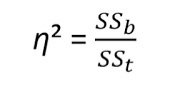
ss_cond = 196.1
ss_total = 196.1 + 297.8
eta_sq <- ss_cond / ss_total

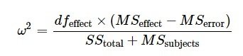
dfeffect = 3
MSeffect = 65.36
MSerror = 5.22
SStotal = 196.1 + 297.8
MSsubjects = 9.242

 

Omega2 = (dfeffect * (MSeffect - MSerror)) / (SStotal + MSsubjects)

Repeated Measures ANOVA

Předpoklady použití

Povaha proměnných

• "Závislá" proměnná kardinální úrovně měření

 

Normalita rozložení závislé proměnné

• V rámci každé sledované skupiny
• Neparametrická alternativa – Friedmanův test

 

Sféricita

• ​Sphericity is the condition where the variances of the differences between all combinations of related groups (levels) are equal
  • Violation of sphericity is when the variances of the differences between all combinations of related groups are not equal.
• The violation of sphericity is serious for the repeated measures ANOVA, with violation causing the test to become too liberal (i.e., an increase in the Type I error rate)

 

Repeated Measures ANOVA

Předpoklady použití

Mauchy's test

# Define the iq data frame
iq <- cbind(RMANOVA$iq[RMANOVA$condition == "8 days"],
            RMANOVA$iq[RMANOVA$condition == "12 days"],
            RMANOVA$iq[RMANOVA$condition == "17 days"],
            RMANOVA$iq[RMANOVA$condition == "19 days"])

 

# Make an mlm object
mlm <- lm(iq ~ 1)

 

# Mauchly's test
mauchly.test(mlm, x = ~ 1)

Repeated Measures ANOVA

Předpoklady použití

# Normalita rozložení

ggplot(data=RMANOVA, aes(RMANOVA$iq)) +
  geom_histogram(breaks=seq(0, 20, by = 2),
                 col="red",
                 aes(fill=..count..)) +
  scale_fill_gradient("Count", low = "green", high = "red")+
  labs(title="Histogram for IQ Gain") +
  labs(x="IQ Gain", y="Count") + theme(legend.position='none')

 

ggplot(RMANOVA, aes(x=iq, fill=condition2)) +
  geom_histogram(position="identity", binwidth=1, alpha=0.5)

Repeated Measures ANOVA

Friedmanův test

friedman.test(iq ~ condition2 | subject2, data = RMANOVA)

Post-Hoc testy

Úvod

Allow for multiple pairwise comparisons without an increase in the probability of a Type I error

 

Používáme, pokud nemáme dopředu jasné hypotézy

• Srovnávají vše se vším – každou skupinu s každou (ale neumí slučovat skupiny jako kontrasty)

Z principu jsou oboustranné

Je jich mnoho – liší se v několika parametrech:

• Konzervativní (Ch. II. typu) versus Liberální (Ch. I. typu)
  • Most liberal = no adjustment
  • Most conservative = adjust for every possible comparison that could be made
• Ne/vhodné pro porušení předpokladu sféricity

Post-Hoc testy

Doporučení podle Fielda (2012)

 Not only does sphericity create problems for the F in repeated-measures  ANOVA, but also it causes some amusing complications for post hoc tests

• The default is to have no adjustment and simply perform a Tukey LSD post hoc test (this is not recommended).
• The second option is a Bonferroni correction (recommended for the reasons mentioned above), and the final option is a Sidak correction, which should be selected if you are concerned about the loss of power associated with Bonferroni corrected values.

Post-Hoc testy

Tukey

# funkce glht

library(multcomp)
posthoc = glht(model3, linfct = mcp(condition2 = "Tukey"))
summary(posthoc)

Post-Hoc testy

Bonferroni

# Pairwise t-test

with(RMANOVA, pairwise.t.test(iq, condition, p.adjust.method = "bonferroni", paired = T))

# glht

summary(glht(model3, linfct=mcp(condition2 = "Tukey")), test = adjusted(type = "bonferroni"))

Post-Hoc testy

Šidák

# dunn.test

install.packages("dunn.test")
library("dunn.test")
dunn.test (x = RMANOVA$iq, g=RMANOVA$condition2, method="sidak", kw=TRUE, label=TRUE,
           wrap=FALSE, table=TRUE, list=FALSE, rmc=FALSE, alpha=0.05)

Kontrasty

Úvod

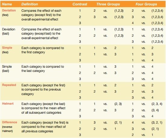
Umožňují porovnat jednotlivé skupiny v jednom kroku bez nutnosti korigovat hladinu významnosti (bez snížení síly testu)

• Jen když máme dopředu hypotézy
• Kontrastů lze provést tolik, kolik je počet skupin – 1

 

Každý kontrast srovnává 2 podmínky

• Průměr skupiny nebo průměr více skupin dohromady
• Např. "19 dnů" vs. "8 dnů" nebo "17 dnů" vs. "12 dnů"

Kontrasty

 

Kontrasty

Příklad

# Helmertův kontrast

options(contrasts = c("contr.helmert", "contr.poly"))
contrasts(RMANOVA$condition2) <- "contr.helmert"
model3 = lme(iq ~ condition2, random = ~1|subject2/condition2, data = RMANOVA, method = "ML")
summary(model3)

Základní literatura

Field, A., Miles, J., & Field, Z. (2012). Discovering Statistics Using R. Sage: UK.

 

Navarro, D. J. (2014). Learning statistics with R: A tutorial for psychology students and other beginners. Available online: http://health.adelaide.edu.au/psychology/ccs/teaching/lsr/