SROVNÁNÍ DVOU PRŮMĚRŮ A JEDNODUCHÁ ANALÝZA SOUVISLOSTI
Vít Gabrhel
vit.gabrhel@mail.muni.cz
FSS MU,
9. 10. 2017

Harmonogram
0. Rekapitulace předchozí hodiny
1. Deskriptivní statistiky - doplnění
2. Srovnání dvou průměrů
3. Chí-kvadrát
4. Korelace
Rekapitulace
Skript
# Jakou třídu (class) tvoří obě proměnné?
class(alco_1$Country)
class(alco_1$Litry)
lapply(Alco, class)
# Změňte tuto hodnotu na "NA"
alco_1$Litry[alco_1$Litry == "-99"] <- NA
Alco$Litry <- str_replace(Alco$Litry,-99.00, "NA")
Alco[46,2] = NA
# Jedna z hodnot je evidentně špatně evidovaná. O jakou hodnotu se jedná?

chyby = subset(alco, subset = (Litry < 0))
# V této nové matici ať jsou všechny země napsané velkými písmeny.
Alco_2 [,"Stát"] = toupper(Alco_2[,"Stát"])


Deskriptivní statistiky
Rozšiřující možnosti
setwd()
library("readxl")
talent_scores_sheets = excel_sheets("talent_scores.xlsx")
talent_scores = read_excel("talent_scores.xlsx", sheet = 1)
# Compute the mean of the scores for each student individually
rowMeans(talent_scores[, 2:6])
# Compute the mean of the scores for each course individually
colMeans(talent_scores[, 2:6])
# Compute the score each student has gained for all his courses
rowSums(talent_scores[, 2:6])
# Compute the total score that is gained by the students on each course
colSums(talent_scores[, 2:6])
Deskriptivní statistiky
Rozšiřující možnosti
wm = read.csv2("wm.csv", header = TRUE)
mean(wm$gain) # function: computes the arithmetic mean
mean(wm$gain, na.rm = TRUE) # function: computes the arithmetic mean
median(wm$gain) # function: computes the median
var(wm$gain) # function: computes the variance
sd(wm$gain) # function: computes the standard deviation
min(wm$gain) # function: return the minimum
max(wm$gain) # function: return the maximum
# Summary statistics for all variables - 5 digits
summary(wm, digits = 5)
# Summary statistics for all variables - 10 digits
summary(wm, digits = 10)
Deskriptivní statistiky
Rozšiřující možnosti
library("dplyr")
# Calculate summary statistics for variables containing "ai". Calculate the statistics to 4 significant digits
summary(select(wm, contains("ai")))
# Alternatively, the numSummary() function might be used to obtain some summary statistics. The function computes:
- mean= the mean
- sd = the standard deviation
- iqr = the interquartile range
- 0% = the minimum
- 25% = the 1st quantile or the lower quartile
- 50% = the median
- 75% = the 3rd quantile or the upper quartile
- 100%= the maximum
- n = the number of observations
library("Rcmdr")
numSummary(wm$gain)
library("Hmisc")
describe(wm)
Korelace
Úvod (dle Pearson product-moment correlation coefficient, n.d.)
Pearson product-moment correlation coeficient
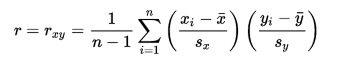
Předpoklady použití:
- Alespoň intervalová úroveň měření proměnných
- Normálně rozložená data
- Homoskedascita
Korelace
base
# Read the variables names
names(talent_scores)
# Create a subset of the dataframe talent, talent_selected, containing reading, english and math (in that order)
talent_selected <- subset(talent_scores, select = c(reading, english, math))
# Předpoklady pro použití
hist(talent_selected$english, main="Histogram for English scores", xlab="Students", border="blue", col="green", xlim=c(0,120), breaks=20)
plot(talent_selected$english, talent_selected$math, main="Scatterplot of Grades", xlab="English ", ylab="Math", pch=19)
qqnorm(talent_selected$math)
Korelace
base
# Compute the correlations among reading, english and math
cor(talent_selected)
#The cor() function does not calculate p-values to test for significance, but the cor.test() function does.
cor.test(talent_selected$english, talent_selected$reading, use = pairwise)
cor.test(talent_selected$reading, talent_selected$math, use = pairwise)
cor.test(talent_selected$english, talent_selected$math, use = pairwise)
Korelace
Rcmdr
# The rcorr.adjust() function of the Rmcdr package computes the correlations with the pairwise p-values among the correlations.
library("Rcmdr")
# Two types of p-values are computed: the ordinary p-values and the adjusted p-values.
?rcorr.adjust
rcorr.adjust(talent_selected)
# Test the significance of the correlations among `english` and `math`
cor.test(talent_selected$english, talent_selected$math, use = pairwise)
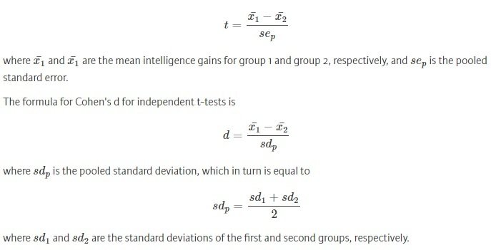
Srovnání dvou průměrů (dle Conway, n.d.)
Dependent t-test - úvod
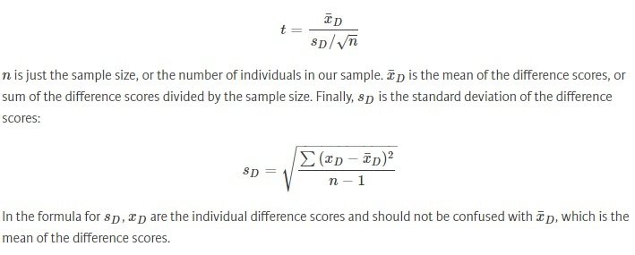
Předpoklady použití:
- The sampling distribution is normally distributed. In the dependent t-
test this means that the sampling distribution of the differences between scores should be normal, not the scores themselves. - Data are measured at least at the interval level.
Srovnání dvou průměrů
Dependent t-test - base - argumenty
# Data
wm_t <- subset(wm, wm$train == "1")
# In the case of our dependent t-test, we need to specify these arguments to t.test():
?t.test
# x: Column of wm_t containing post-training intelligence scores
# y: Column of wm_t containing pre-training intelligence scores
# paired: Whether we're doing a dependent (i.e. paired) t-test or # # independent t-test. In this example, it's TRUE
# Note that t.test() carries out a two-sided t-test by default
Srovnání dvou průměrů
Dependent t-test - base - kód
# Conduct a paired t-test using the t.test function
t.test(wm_t$post, wm_t$pre, paired = TRUE)
Output:
Paired t-test
data: wm_t$post and wm_t$pre
t = 14.492, df = 79, p-value < 2.2e-16
alternative hypothesis: true difference in means is not equal to 0
95 percent confidence interval:
3.008511 3.966489
sample estimates:
mean of the differences
3.4875

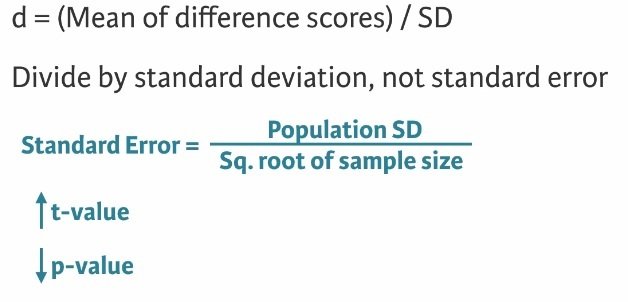
Srovnání dvou průměrů (dle Conway, n.d.)
Dependent t-test - Cohenovo d
Srovnání dvou průměrů
Dependent t-test - Cohenovo d - lsr - argumenty
library("lsr")
# For cohensD(), we'll need to specify three arguments:
# x: Column of wm_t containing post-training intelligence scores
# y: Column of wm_t containing pre-training intelligence scores
# method: Version of Cohen's d to compute, which should be "paired" in this case
?cohensD()
Srovnání dvou průměrů
Dependent t-test - Cohenovo d - lsr - output
# Calculate Cohen's d
cohensD(wm_t$post, wm_t$pre, method = "paired")
[1] 1.620297
Srovnání dvou průměrů
Dependent t-test - Cohenovo d - effsize - argumenty
library("effsize")
cohen.d(x, y, pooled=TRUE, paired=TRUE,
na.rm=FALSE, hedges.correction=FALSE,
conf.level=0.95, noncentral=FALSE)
?cohen.d()
Srovnání dvou průměrů
Dependent t-test - Cohenovo d - effsize - příklad
library("effsize")
cohen.d(wm_t$post,wm_t$pre,pooled=TRUE,paired=TRUE,
na.rm=FALSE, hedges.correction=FALSE,
conf.level=0.95,noncentral=FALSE)

Srovnání dvou průměrů (dle Conway, n.d.)
Independent t-test - úvod
Předpoklady použití:
- The sampling distribution is normally distributed.
- Data are measured at least at the interval level.
- Homogeneity of variance.
- Scores are independent (because they come from different people).
Srovnání dvou průměrů
Independent t-test - data
# View the wm_t dataset
wm_t
# Create subsets for each training time
wm_t08 <- subset(wm_t, subset = (wm_t$cond == "t08"))
wm_t12 <- subset(wm_t, subset = (wm_t$cond == "t12"))
wm_t17 <- subset(wm_t, subset = (wm_t$cond == "t17"))
wm_t19 <- subset(wm_t, subset = (wm_t$cond == "t19"))
# Summary statistics for the change in training scores before and after training
describe(wm_t08)
describe(wm_t12)
describe(wm_t17)
describe(wm_t19)
# Create a boxplot of the different training times
ggplot(wm_t, aes(x = cond, y = gain, fill = cond)) + geom_boxplot()
# Levene's test
leveneTest(wm_t$gain ~ wm_t$cond)
Srovnání dvou průměrů
Independent t-test - base
# Conduct an independent t-test
t.test(wm_t19$gain, wm_t08$gain, var.equal = FALSE)
Welch Two Sample t-test
data: wm_t19$gain and wm_t08$gain
t = 8.9677, df = 34.248, p-value = 1.647e-10
alternative hypothesis: true difference in means is not equal to 0
95 percent confidence interval:
3.287125 5.212875
sample estimates:
mean of x mean of y
5.60 1.35
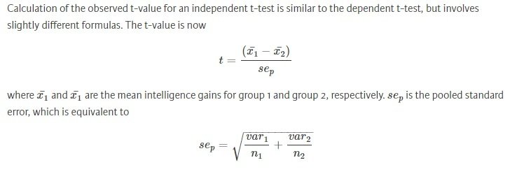
Srovnání dvou průměrů (dle Conway, n.d.)
Independent t-test - Cohen's d
Srovnání dvou průměrů
Independent t-test - effsize
# Calculate Cohen's d
cohen.d(wm_t19$gain, wm_t08$gain,pooled=TRUE,paired=FALSE,
na.rm=FALSE, hedges.correction=FALSE,
conf.level=0.95,noncentral=FALSE)
Cohen's d
d estimate: 2.835822 (large)
95 percent confidence interval:
inf sup
1.893561 3.778083
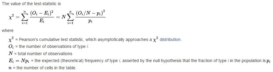
Chí-kvadrát (dle Pearson's chi-squared test, n.d.)
Úvod
Předpoklady použití:
-
Ne méně než 20 % buněk v rámci kontigenční tabulky s hodnotou méně než 5
-
Nenulová hodnota v každé z buněk v rámci kontingenční tabulky
Chí-kvadrát
Data a gmodels
# Data
- gedu_sheets = excel_sheets("gedu.xlsx")
- gedu = read_excel("gedu.xlsx", sheet = 1)
- gedu$Gender = as.factor(gedu$Gender)
- gedu$Edu = as.factor(gedu$Edu)
- gedu$Edu2 = as.factor(gedu$Edu2)
- levels(gedu$Gender) = c("Muž", "Žena")
- levels(gedu$Edu) = c("ZŠ", "SŠ bez maturity", "SŠ s maturitou", "VŠ")
- levels(gedu$Edu2) = c("Nižší než VŠ", "VŠ")
# gmodels
library("gmodels")
?CrossTable()
Chí-kvadrát
Kontingenční tabulky
# Generate a cross table of gender and education
Gedu_CT_01 <- CrossTable(gedu$Edu, gedu$Gender)
# Generate a crosstable for gender and education in which only the results for the chi-square test are included, and the row proportions.
Gedu_CT_02 = CrossTable(gedu$Edu, gedu$Gender, prop.c = FALSE, prop.t = FALSE, chisq = TRUE, prop.chisq = FALSE)
# Generate a cross table of gender and fulltime in SPSS format
Gedu_CT_03 = CrossTable(gedu$Edu, gedu$Gender, format = "SPSS")
Chí-kvadrát
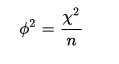
Velikost účinku - phí (dle Phi coefficient, n.d.)
library("psych")
Gen = gedu$Gender
Edu2 = gedu$Edu2
table_phi = table(Gen, Edu2)
phi(table_phi, digits = 2)
Chí-kvadrát
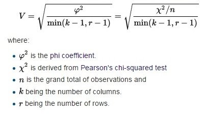
Velikost účinku - Cramerovo V (dle Cramér's V, n.d.)
library("psych")
Gen = gedu$Gender
Edu = gedu$Edu
table_CV = table(Gen, Edu)
cramersV(table_CV)

Zdroje
Conway, A. (n.d.) Intro to Statistics with R: Student's T-test. Dostupné online na: https://www.datacamp.com/courses/intro-to-statistics-with-r-students-t-test
Cramér's V. (n.d.). In Wikipedia: Staženo dne 10. 10. 2016 z https://en.wikipedia.org/wiki/Cram%C3%A9r%27s_V
Effect size (n.d.). In Wikipedia: Staženo dne 10. 10. 2016 z https://en.wikipedia.org/wiki/Effect_size
Pearson's chi-squared test (n.d.). In Wikipedia: Staženo dne 10. 10. 2016 z https://en.wikipedia.org/wiki/Pearson%27s_chi-squared_test
Pearson product-moment correlation coefficient (n.d.). In Wikipedia: Staženo dne 10. 10. 2016 z https://en.wikipedia.org/wiki/Pearson_product-moment_correlation_coefficient
Phi coefficient (n.d.). In Wikipedia: Staženo dne 10. 10. 2016 z https://en.wikipedia.org/wiki/Phi_coefficient
Sampling distribution (n.d.). In Wikipedia: Staženo dne 10. 10. 2016 z https://en.wikipedia.org/wiki/Sampling_distribution
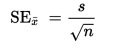
Standard error (n.d.). In Wikipedia: Staženo dne 10. 10. 2016 z https://en.wikipedia.org/wiki/Standard_error
Student's t-test (n.d.). In Wikipedia: Staženo dne 10. 10. 2016 z https://en.wikipedia.org/wiki/Student%27s_t-test