Loss Landscape and
Performance in Deep Learning
M. Geiger, A. Jacot, S. d’Ascoli, M. Baity-Jesi,
L. Sagun, G. Biroli, C. Hongler, M. Wyart
Stefano Spigler
arXivs: 1901.01608; 1810.09665; 1809.09349

(Supervised) Deep Learning
\(<-1\)
\(>+1\)
- Learning from examples: train set
- Is able to predict: test set
- Not understood why it works so well!
\(f(\mathbf{x})\)

-
How many data are needed to learn?
- What network size?
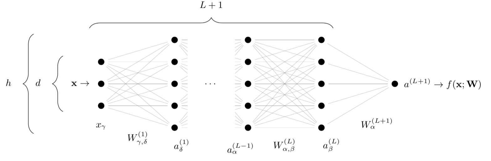
Set-up: Architecture
- Deep net \(f(\mathbf{x};\mathbf{W})\) with \(\textcolor{red}{N}\sim h^2L\) parameters
depth \(L\)
width \(\color{red}h\)
\(f(\mathbf{x};\mathbf{W})\)
- Alternating linear and nonlinear operations!
\(W_\mu\)
Set-up: Dataset
- \(\color{red}P\) training data:
\(\mathbf{x}_1, \dots, \mathbf{x}_P\)
- Binary classification:
\(\mathbf{x}_i \to \mathrm{label}\ y_i = \pm1\)
- Independent test set to evaluate performance
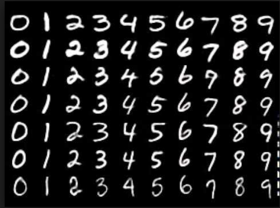
Example - MNIST (parity):
70k pictures, digits \(0,\dots,9\);
use parity as label
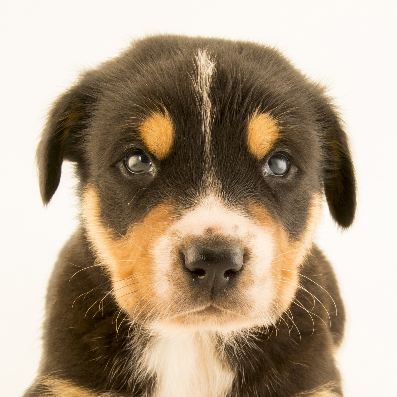
\(\pm1=\) cats/dogs, yes/no, even/odd...
Outline
Vary network size \(\color{red}N\) (\(\sim\color{red}h^2\)):
- Can networks fit all the \(\color{red}P\) training data?
- Can networks overfit? Can \(\color{red}N\) be too large?
\(\to\) Long term goal: how to choose \(\color{red}N\)?
\(h\)
Learning
-
Find parameters \(\mathbf{W}\) such that \(\mathrm{sign} f(\mathbf{x}_i; \mathbf{W}) = y_i\) for \(i\in\) train set
-
Minimize some loss!
-
\(\mathcal{L}(\mathbf{W}) = 0\) if and only if \(y_i f(\mathbf{x}_i;\mathbf{W}) > 1\) for all patterns
(classified correctly with some margin)

Binary classification: \(y_i = \pm1\)
Hinge loss:
Learning dynamics = descent in loss landscape
-
Minimize loss \(\longleftrightarrow\) gradient descent
-
Start with random initial conditions!
Random, high dimensional, not convex landscape!
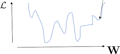
- Why not stuck in bad local minima?
- What is the landscape geometry?
- Many flat directions are found!
bad local minimum?
Soudry, Hoffer '17; Sagun et al. '17; Cooper '18; Baity-Jesy et al. '18 - arXiv:1803.06969
in practical settings:
Analogy with granular matter: Jamming
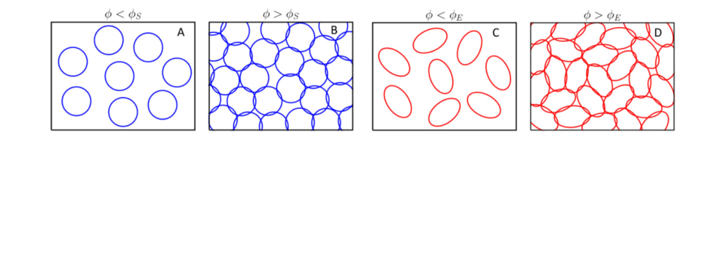
Upon increasing density \(\to\) transition
sharp transition with finite-range interactions
- random initial conditions
- minimize energy \(\mathcal{L}\)
- either find \(\mathcal{L}=0\) or \(\mathcal{L}>0\)
Random packing:
this is why we use the hinge loss!
Shallow networks \(\longleftrightarrow\) packings of spheres: Franz and Parisi, '16
Deep nets \(\longleftrightarrow\) packings of ellipsoids!
(if signals propagate through the net)
\(\color{red}N^\star < c_0 P\)
typically \(c_0=\mathcal{O}(1)\)

Theoretical results: Phase diagram
- When \(N\) is large, \(\mathcal{L}=0\)
- Transition at \(N^\star\)
\(\color{red}N^\star < c_0 P\)
\(\color{red}N^\star\)
network size
dataset size
Empirical tests: MNIST (parity)
Geiger et al. '18 - arXiv:1809.09349;
Spigler et al. '18 - arXiv:1810.09665
- Above \(\color{red}N^*\) we have \(\mathcal{L}=0\)
- Solid line is the bound \(\color{red}N^* < c_0 P\)
No local minima are found when overparametrized!
\(P\)
\(N\)
dataset size
network size
\(\color{red}N^\star < c_0 P\)
Landscape curvature
Spectrum of the Hessian (eigenvalues)
We don't find local minima when overparametrized... ...shape of the landscape?
Geiger et al. '18 - arXiv:1809.09349
Local curvature:
second order approximation

Information captured by Hessian matrix: \(\mathcal{H}_{\mu\nu} = \frac{\partial^2}{\partial_{\mathbf{W}_\mu}\partial_{\mathbf{W}_\nu}} \mathcal{L}(\mathbf{W})\)
w.r.t parameters \(W\)
Flat directions
Spectrum
Over-parametrized
Jamming
Under-parametrized
\(\sim\sqrt{\mathcal{L}}\)


\(\leftrightarrow\)
eigenvalues
eigenvalues
eigenvalues
\(\mathcal{L} = 0\)
Flat
Geiger et al. '18 - arXiv:1809.09349
Almost flat

\(N>N^\star\)
\(N\approx N^\star\)
\(N<N^\star\)
Spectrum
Spectrum
From numerical simulations:
(at the transition)
Dirac \(\delta\)'s
depth
Outline
Vary network size \(\color{red}N\) (\(\sim\color{red}h^2\)):
- Can networks fit all the \(\color{red}P\) training data?
- Can networks overfit? Can \(\color{red}N\) be too large?
\(\to\) Long term goal: how to choose \(\color{red}N\)?
\(h\)
Yes, deep networks fit all data if \(N>N^*\ \longrightarrow\) jamming transition
Generalization
Spigler et al. '18 - arXiv:1810.09665
Ok, so just crank up \(N\) and fit everything?
Generalization? \(\to\) Compute test error \(\epsilon\)
But wait... what about overfitting?
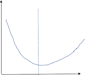
overfitting
\(N\)
\(N^*\)
Test error \(\epsilon\)

Train error
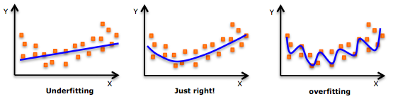
example: polynomial fitting
\(N \sim \mathrm{polynomial\ degree}\)
Overfitting?
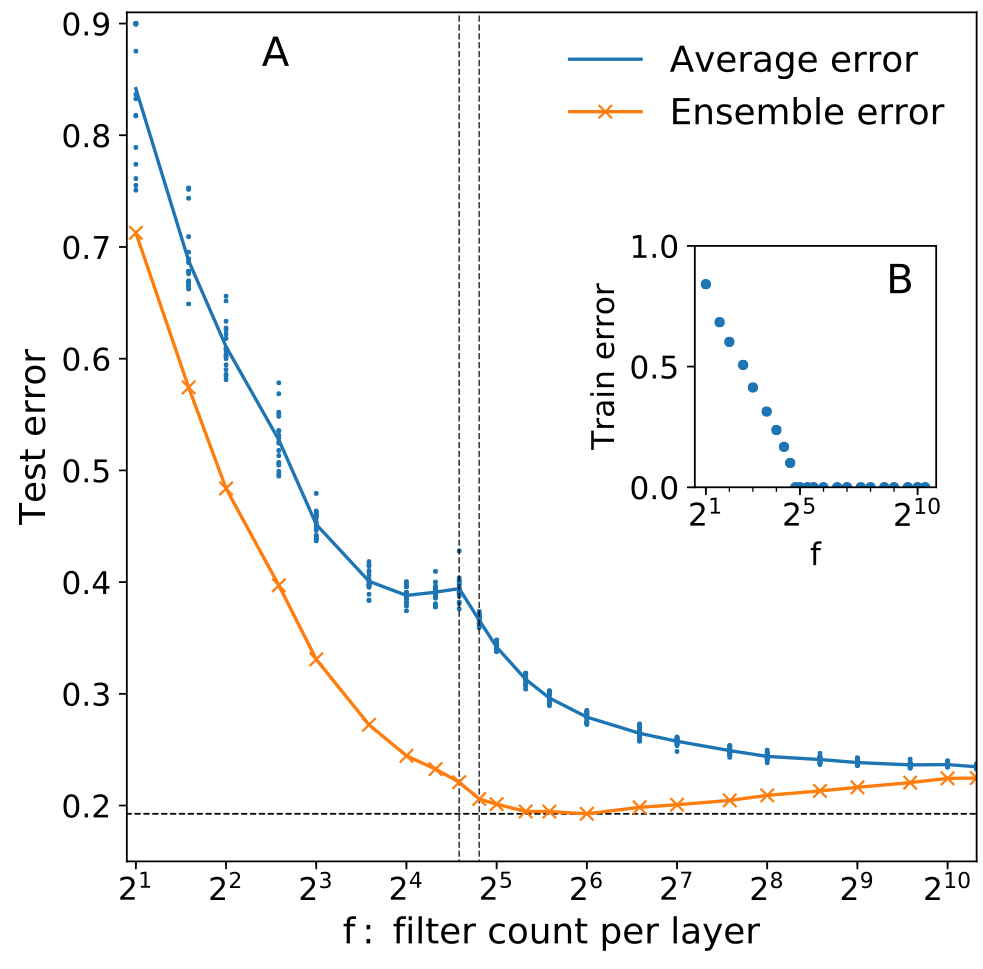
Spigler et al. '18 - arXiv:1810.09665
-
Test error decreases monotonically with \(N\)!
- Cusp at the jamming transition
Advani and Saxe '17;
Spigler et al. '18 - arXiv:1810.09665;
Geiger et al. '19 - arXiv:1901.01608
"Double descent"

test error
\(N\)
\(N/N^*\)
(after the peak)
\(P\)
\(N\)
dataset size
network size
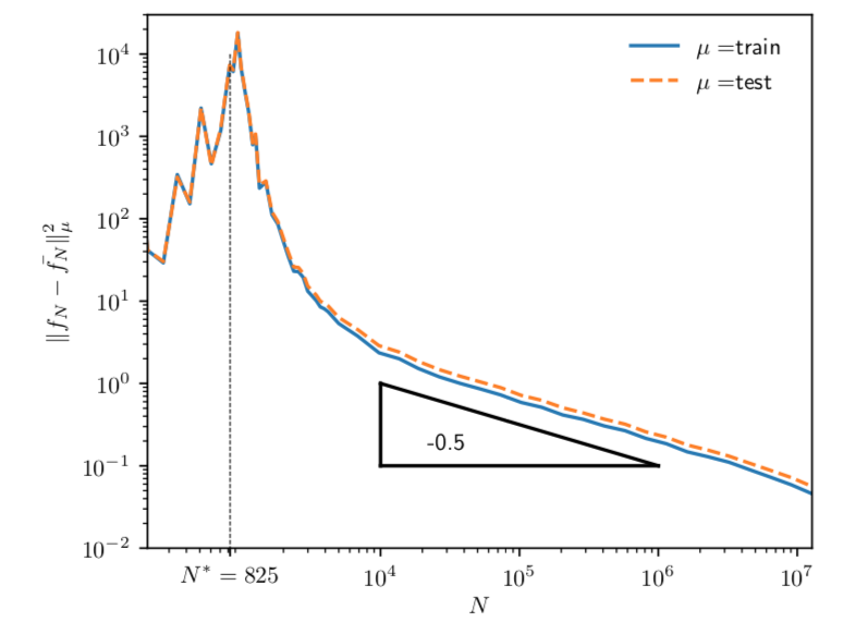
We know why: Fluctuations!
Ensemble average
- Random initialization \(\to\) output function \(f_{\color{red}N}\) is stochastic
- Fluctuations: quantified by average and variance
ensemble average over \(n\) instances:
\(\phantom{x}\)
\(f_N(\mathbf{W}_1)\)
\(f_N(\mathbf{W}_2)\)
\(f_N(\mathbf{W}_3)\)


\(-1\)
\(-1\)
\(+1\)
\(\bar f_N\)
\(-1!\)
\(\frac{{\color{red}-1-1}{\color{blue}+1}}{3}\cdots\)
Explained in a few slides
Define some norm over the output functions:
ensemble variance (fixed \(n\)):
\(\phantom{x}\)
Fluctuations increase error
\( \{f(\mathbf{x};\mathbf{W}_\alpha)\} \to \left\langle\epsilon_N\right\rangle\)
Remark:
Geiger et al. '19 - arXiv:1901.01608

-
Test error increases with fluctuations
- Ensemble test error is nearly flat after \(N^*\)!
\(\bar f^n_N(\mathbf{x}) \to \bar\epsilon_N\)
test error of ensemble average
average test error
\(\neq\)
normal average
ensemble average
test error \(\epsilon\)
test error \(\epsilon\)
(CIFAR-10 \(\to\) regrouped in 2 classes)
(MNIST parity)
Scaling argument!
Geiger et al. '19 - arXiv:1901.01608
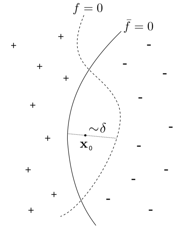
decision boundaries:
Smoothness of test error as function of decision boundary + symmetry:
normal average
ensemble average
Infinitely-wide networks: Initialization
Neal '96; Williams '98; Lee et al '18; Schoenholz et al. '16
- Weights: each initialized as \(W_\mu\sim {\color{red}h}^{-\frac12}\mathcal{N}(0,1)\)
- Neurons sum \(\color{red}h\) signals of order \({\color{red}h}^{-\frac12}\) \(\longrightarrow\) Central Limit Theorem
- Output function becomes a Gaussian Random Field
width \(\color{red}h\)
\(f(\mathbf{x};\mathbf{W})\)
input dim \(\color{red}d\)
\(W^{(1)}\sim d^{-\frac12}\mathcal{N}(0,1)\)
as \(h\to\infty\)
\(W_\mu\)
Infinitely-wide networks: Learning
Jacot et al. '18
- For small width \(h\): \(\nabla_{\mathbf{W}}f\) evolves during training
- For large width hh\(h\): \(\nabla_{\mathbf{W}}f\) is constant during training
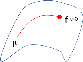
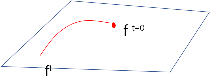
For an input the function lives on a curved manifold
The manifold becomes linear!
Lazy learning:
- weights don't change much:
- enough to change the output \(f\) by \(\sim \mathcal{O}(1)\)!\partial_{\mathbf{W}}
Neural Tangent Kernel
- Gradient descent implies:
The formula for the kernel \(\Theta^t\) is useless, unless...
Theorem. (informal)
Deep learning \(=\) learning with a kernel as \(h\to\infty\)
Jacot et al. '18
\(\phantom{x}\)
convolution with a kernel
\(\phantom{wwwwwwww}\)
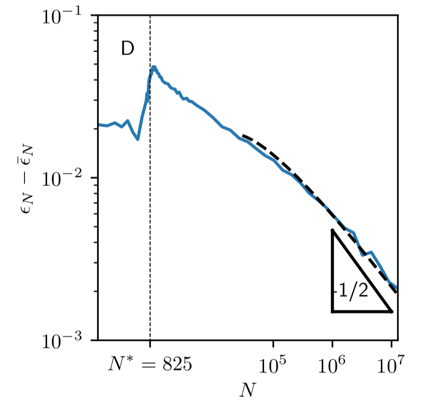
Finite \(N\) asymptotics?
Geiger et al. '19 - arXiv:1901.01608;
Hanin and Nica '19;
Dyer and Gur-Ari '19
-
Evolution in time is small:
- Fluctuations are much larger:
Then:
The output function fluctuates similarly to the kernel
\(\Delta\Theta^{t=0} \sim 1/\sqrt{h} \sim N^{-\frac14}\)
at \(t=0\)
\(|\!|\Theta^t - \Theta^{t=0}|\!|_F \sim 1/h \sim N^{-\frac12}\)
Conclusion
1. Can networks fit all the \(\color{red}P\) training data?
-
Yes, deep networks fit all data if \(N>N^*\ \longrightarrow\) jamming transition
-
Initialization induces fluctuations in output that increase test error
- No overfitting: error keeps decreasing past \(N^*\) because fluctuations diminish
check Geiger et al. '19 - arXiv:1906.08034 for more!
check Spigler et al. '19 - arXiv:1905.10843 !
2. Can networks overfit? Can \(\color{red}N\) be too large?
3. How does the test error scale with \(\color{red}P\)?
\(\to\) Long term goal: how to choose \(\color{red}N\)?
(tentative) Right after jamming, and do ensemble averaging!