Theory of Everything
Graph Signal Processing
with application to scRNA-seq
Quantifying the effect of experimental perturbations in single-cell RNA-sequencing data using graph signal processing


Quantifying the effect of experimental perturbations in single-cell RNA-sequencing data using graph signal processing
def filterfunc(x):
    return (np.exp(-b * np.abs(x / graph.lmax - a)**p))

filt = pygsp.filters.Filter(graph, filterfunc)
EES = filt.filter(RES, method="chebyshev", order=50)

Graph Signal Processing:
Overview, Challenges and Applications


Quick plan
-
Spectral Graph Theory: study graph properties. Here I'll explain some existing algorithms.
- Graph Signal Processing: study signals on graphs. Here I'll propose some new algorithms, including the mentioned paper.
Intro to Spectral Graph Theory
Intro to Spectral Graph Theory
Questions:
- Who remembers what are eigenvalues?
- Who knows what is Fourier Transform?
- Who knows what the Laplace Operator (∆) does?


- Markov Random Fields
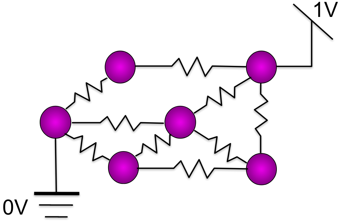
- Electrical chains
- Heat diffusion
- Finite element method
- Google PageRank algorithm
- Random Walks on graphs
- Spectral clustering
- Pseudo-time ordering of cells
- DiffusionMap visualization
- Conos annotation transfer
What do all these processes have in common?
Intro to Spectral Graph Theory
Why should you even care?
Intro to Spectral Graph Theory
Why should you even care?
void smooth_cm(const std::vector<Edge> &edges, Mat &cm,
               int max_n_iters, double c, double f, double tol,
               const std::vector<bool> &is_label_fixed) {
  std::vector<double> sum_weights(cm.rows(), 1);
  for (int iter = 0; iter < max_n_iters; ++iter) {
    Mat cm_new(count_matrix);
    for (auto const &e : edges) {
      double weight = exp(-f * (e.length + c));
      if (is_label_fixed.empty() || !is_label_fixed.at(e.v_start)) {
        cm_new.row(e.v_start) += cm.row(e.v_end) * weight;
      }

      if (is_label_fixed.empty() || !is_label_fixed.at(e.v_end)) {
        cm_new.row(e.v_end) += cm.row(e.v_start) * weight;
      }
    }

    double inf_norm = (cm_new - cm).array().abs().matrix().lpNorm<Infinity>();
    if (inf_norm < tol)
      break;

    cm = cm_new;
  }
}- Markov Random Fields
- Electrical chains
- Heat diffusion
- Finite element method
- Google PageRank algorithm
- Random Walks on graphs
- Spectral clustering
- Pseudo-time ordering of cells
- DiffusionMap visualization
- Conos annotation transfer
What do all these processes have in common?
Some examples
Gene networks
0
1
Associated with disease
No association with disease
0.5
0.375
0.625
0.5
Markov Random Field

Minimize
Some examples
Electrical networks

0V
1V
0.5
0.325
0.675
0.5
Potentials
Minimize
Some examples
Quadratic form minimization
Minimize over x
Quadratic form
1V

0.5
0.5
0.325
0.675
0V
Graph Laplacian
System of linear equations
Applying the operator
creates some flow on the graph
It's all about Laplacian
: degree matrix
: adjacency matrix
Non-Normalized Graph Laplacian:
Connection to the Laplace Operator
Finite element method

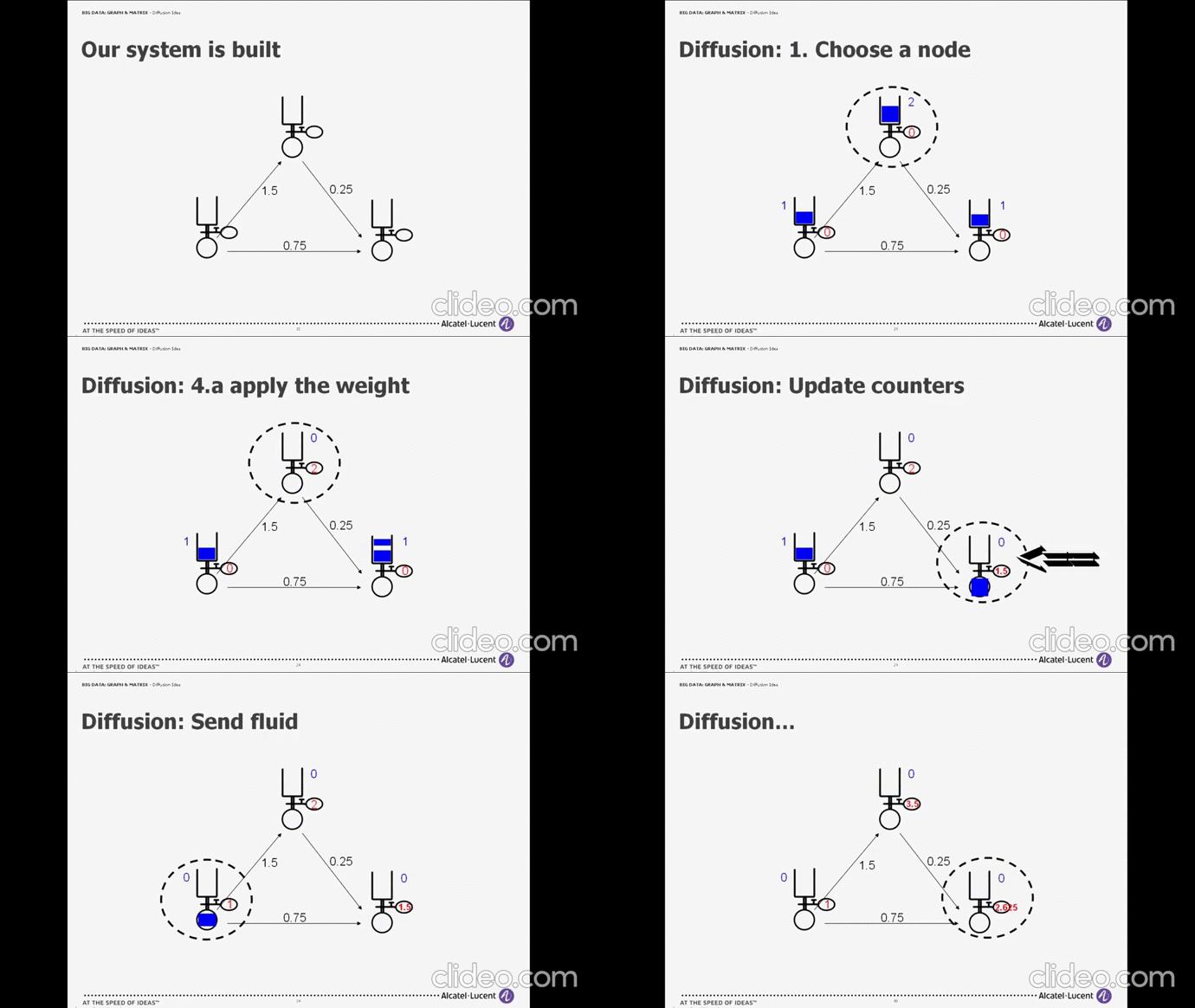
Laplace Operator:
Heat Equation:
Informally, the Laplacian operator ∆ gives the difference between the average value of a function in the neighborhood of a point, and its value at that point. [wiki]
Graph diffusion:
Other graph matrices:
Adjacency matrix
Normalized Laplacian
Random walk matrix
...
Other ways to define flow on graphs
: degree matrix
: adjacency matrix
Non-Normalized Graph Laplacian:
Practical applications
Pseudotime estimation**


Conos Annotation Transfer
Google PageRank algorithm*
k-NN Smoothing
(no picture)
Practical applications
Pseudotime estimation**


Conos Annotation Transfer
Google PageRank algorithm*
k-NN Smoothing
(no picture)
Can we re-write the Velocity equations on graph?
Eigenvalues of the Laplacian matrix
Eigenvalues:
Eigenvectors:
Eigenvalues of the Laplacian matrix
Courant-Fisher Theorem
is a constant vector
Connected nodes have close vector values!
Eigenvalues of the Laplacian matrix
Spectral Drawing

Eigenvalues of the Laplacian matrix
Spectral Drawing

emb <- uwot::umap(
    X,
    metric="cosine",
    init="spectral"
)
Eigenvalues of the Laplacian matrix
Diffusion Map
Normalized Laplacian
Normalized Laplacian Random walk matrix
Non-Normalized Laplacian
Laplacian
Degree matrix
Spectral drawing
Connected to Hitting Distances on graph
Eigenvalues of the Laplacian matrix
Spectral Clustering and Min Cut


k-Means in spectral space approximates Minimum k-cut
Practical applications
- Spectral visualization
- Diffusion Maps
- Spectral clustering
- Fast Minimal Cuts
Graph Signal Processing
- Aviyente, S. et. al. "Cooperative and Graph Signal Processing" (2018)
- Shuman, D. I. et al. "The Emerging Field of Signal Processing on Graphs: Extending High-Dimensional Data Analysis to Networks and Other Irregular Domains." (2013)
- Ortega, A. et. al. "Graph Signal Processing: Overview, Challenges, and Applications" (2018)
Signals on graphs
Example: Gene expression as a signal

Signals on graphs
Alternative view on the Quadratic Form
Signal is given over the graph domain.
Derivative over an edge:
Gradient:
Local variation:
Laplacian:
Signals on graphs
Alternative view on the Quadratic Form
Local variation:
Global variation:
Signals on graphs
Possible application: measure alignment quality
Local variation:
Global variation:
-
Signal = Expression: we can measure local / global variation of expression after the alignment and compare it to the variation before
- Signal = Sample labels: we can measure local variation of samples
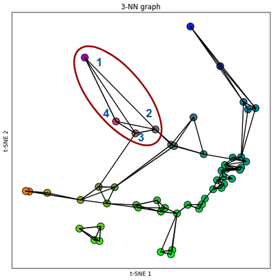

Example: Gene expression as a signal
k-NN smoothing is noise filtering
Image filtering


Image filtering


Filter size = k-hop on graph
Can we increase k?
Grid = Graph
Image filtering
Fourier Transform

- Represents signal as a combination of waves
- Spectral domain: frequency vs amplitude
- Every pixel has some info from every other pixel
- We can work with frequencies!
- Fast Fourier Transform: O(N log N)

Image filtering
Spectral Domain Filters

Low-pass filter*


High-pass filter**
Fourier transform on graphs
For eigenvector :
Global variation:

Fourier transform on graphs
Inverse Fourier transform of :
Fourier transform of :
For eigenvector :
Global variation:
Fourier transform on graphs
Function projections on frequencies
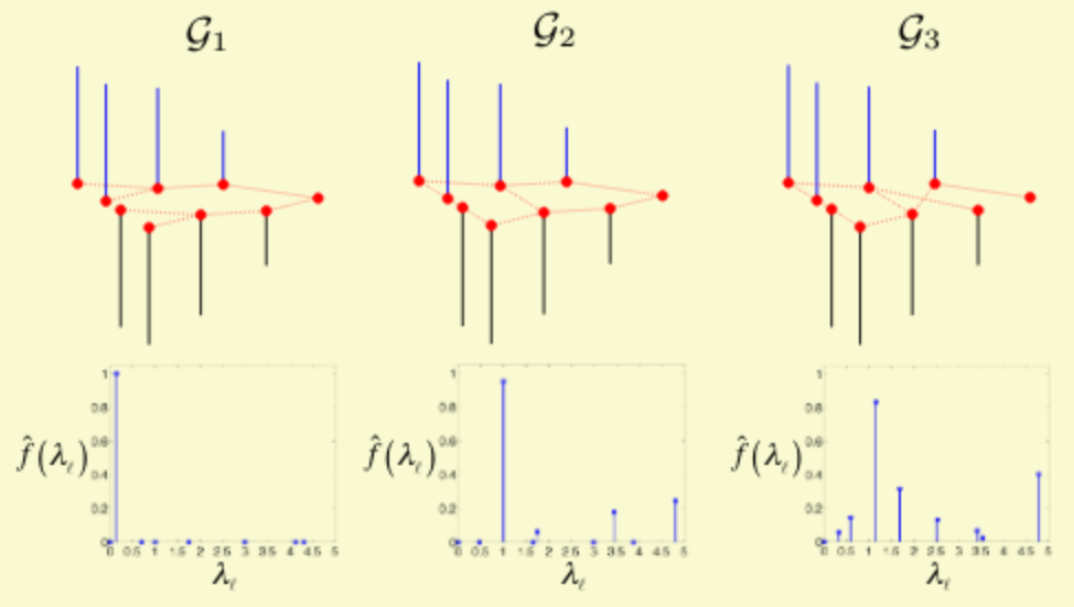
Fourier transform on graphs
General definition of filters
Inverse Fourier transform of :
Applying a
spectral filter :
Fourier transform on graphs
Example: Tikhonov regularization
It's just a low-pass filter
Fourier transform on graphs
Computational problems
- Direct Fourier transform takes
- We can do a polynomial approximation for
Possible application
Tikhonov regularization for expression correction?
- We can use Tikhonov regularization as for correcting batch effect using the Conos graph
- Gamma is a correction strength
- We can determine it comparing corrected expression variation to expression variation of individual samples
Filters on graphs
Back to images

Low-pass filter*


High-pass filter**
MELD: low-pass filter
def filterfunc(x):
    return (np.exp(-b * np.abs(x / graph.lmax - a)**p))

filt = pygsp.filters.Filter(graph, filterfunc)
EES = filt.filter(RES, method="chebyshev", order=50)
MELD: low-pass filter


Other filter parameters


Other filter parameters


Possible applications
- Whatever we need to smooth, low-pass filters work much better than k-NN smoothing.
- Low-pass filters are a proper way for Kernel Density Estimation on graphs. We can at least apply it to estimate density of healthy vs control samples for cross-condition comparison.
- Can we use high-pass filters over expression to detect cell type boundaries? :)
Other signal transformations

Translation
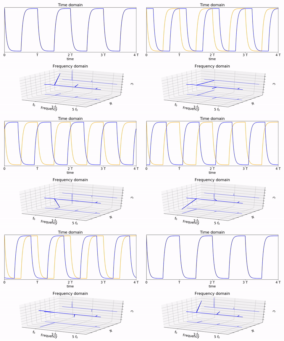
Modulation

Convolution

Dilation
Other signal transformations
Down-sampling

Other signal transformations
Down-sampling

We can down-sample graph (both vertices and edges), preserving both graph topology and the signal!
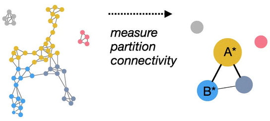
We can do a better PAGA:
Other signal transformations
- Wavelet analysis (on the example of hierarchical subtraction)
- Time-vertex domain: graph is one dimension and time is another
- Random Processes on graphs
Multiscale Wavelet Analysis


