PREPROCESSING 102
#NLP
Challenge #2
https://www.kaggle.com/c/cnam-niort-20192020/data
Deadline challenge & rapport : 5 avril
Outline
- Basics
- Count Features
- Tf-IDF
- N-Grams
- Dense vectors
- Word2Vec
- GloVe
- Deep learning & NLP
Basics
Library NLTK
import nltk
nltk.download()
Tokenize
from nltk.tokenize import sent_tokenize, word_tokenize
# Best for European languages

text = "Hey Bob! What's the weather at 8 o'clock"
sent_tokenize(text)
# ['Hey Bob!', "What's the weather at 8 o'clock"]
word_tokenize(sent_tokenize(text)[1])
# ['What', "'s", 'the', 'weather', 'at', '8', "o'clock"]
Part Of Speech Tagging
tokens = word_tokenize("I went to Paris to meet Bob")
nltk.pos_tag(tokens)
# [('I', 'PRP'),
#  ('went', 'VBD'),
#  ('to', 'TO'),
#  ('Paris', 'NNP'),
#  ('to', 'TO'),
#  ('meet', 'VB'),
#  ('Bob', 'NNP')]

nltk.ne_chunk(nltk.pos_tag(tokens), binary=True)
# Tree('S', [
#     ('I', 'PRP'), ('went', 'VBD'), ('to', 'TO'),
#     Tree('NE', [('Paris', 'NNP')]), ('to', 'TO'), ('meet', 'VB'),
#     Tree('NE', [('Bob', 'NNP')]),
# ])
POS tagger in NLTK isn't that great, if you want a good model, take a look at SyntaxNet
Stemming
Word -> Stem (non-changing portion)
# The two most used stemmers
from nltk.stem import SnowballStemmer
from nltk.stem.porter import PorterStemmer

snow = SnowballStemmer('english')

snow.stem("own") == snow.stem("owning") == snow.stem("owned")
# True

snow.stem("entities") == snow.stem("entity")
# True
Velocity: Snowball > Porter
Perf: Porter > Snowball
Lemmatisation
Word -> Lemma (dictionary form)
from nltk.stem import WordNetLemmatizer

wordnet = WordNetLemmatizer()

wordnet.lemmatize("women")
# u'woman'

wordnet.lemmatize("marketing")
# 'marketing'

wordnet.lemmatize("markets")
# u'market'

snow.stem("marketing")
# u'market'

snow.stem("markets")
# u'market'
/!\ Really slow /!\
Stop Words
from nltk.corpus import stopwords

len(stopwords.words('english'))
# 153

stopwords.words('english')[:20]
# [u'i',
#  u'me',
#  u'my',
#  u'myself',
#  u'we',
#  u'our',
#  u'ours',
#  u'ourselves',
#  u'you',
#  u'your',
#  u'yours',
#  u'yourself',
#  u'yourselves',
#  u'he',
#  u'him',
#  u'his',
#  u'himself',
#  u'she',
#  u'her',
#  u'hers']
String Metrics
Most widely used:
- Levenshtein distance (+++)
- minimum number of character edits (insert, delete, substitue) to go from one word to the other
- Jaro-Winkler distance
- Kinda the same but give more importance to the beginning of a word
Basic TODO
- Lowercase
- Normalize the punctuation; whatever your way, eg:
- after a comma, always a space
- every punctuation is turned to a space
- Normalize spaces: multiple to single
- Non-ASCII to ASCII: special characters, accents
Count Features
Count Vectorizer
Input: Corpus of text documents
Output: Matrix NxM with N = # of documents, M = # of unique words
from sklearn.feature_extraction.text import CountVectorizer

corpus = [
     'This is the first document.',
     'This is the second second document.',
     'And the third one.',
     'Is this the first document?',
 ]
vectorizer = CountVectorizer()
vectorizer.fit_transform(corpus).toarray()
# array([[0, 1, 1, 1, 0, 0, 1, 0, 1],
#        [0, 1, 0, 1, 0, 2, 1, 0, 1],
#        [1, 0, 0, 0, 1, 0, 1, 1, 0],
#        [0, 1, 1, 1, 0, 0, 1, 0, 1]])

vectorizer.get_feature_names()
# [u'and', u'document', u'first', u'is', u'one', u'second',
# u'the', u'third', u'this']
TF-IDF
Normalization of occurrence matrix:
Frequency of a word in a document, weighted by its rarity in the corpus
tf: reward for high occurrence in a document
idf: penalty if too much appearance in the corpus
(log term because, most of the time, words distribution across a corpus is a power law)
TF-IDF
import numpy as np
from sklearn.feature_extraction.text import TfidfVectorizer

corpus = [
     'This is the first document.',
     'This is the second second document.',
     'And the third one.',
     'Is this the first document?',
 ]
vectorizer = TfidfVectorizer()
np.around(vectorizer.fit_transform(corpus).toarray(), decimals=2)

# array([[ 0.  ,  0.44,  0.54,  0.44,  0.  ,  0.  ,  0.36,  0.  ,  0.44],
#        [ 0.  ,  0.27,  0.  ,  0.27,  0.  ,  0.85,  0.22,  0.  ,  0.27],
#        [ 0.55,  0.  ,  0.  ,  0.  ,  0.55,  0.  ,  0.29,  0.55,  0.  ],
#        [ 0.  ,  0.44,  0.54,  0.44,  0.  ,  0.  ,  0.36,  0.  ,  0.44]])

vectorizer.get_feature_names()
# [u'and', u'document', u'first', u'is', u'one', u'second',
# u'the', u'third', u'this']
N-Grams
from sklearn.feature_extraction.text import CountVectorizer

text = "word1 word2 word3 word4 word5"
CountVectorizer(ngram_range=(1,4)).build_analyzer()(text)
# [u'word1',
#  u'word2',
#  u'word3',
#  u'word4',
#  u'word5',
#  u'word1 word2',
#  u'word2 word3',
#  u'word3 word4',
#  u'word4 word5',
#  u'word1 word2 word3',
#  u'word2 word3 word4',
#  u'word3 word4 word5',
#  u'word1 word2 word3 word4',
#  u'word2 word3 word4 word5']


# Do the same, just with Python
def find_ngrams(input_list, n):
  return zip(*[input_list[i:] for i in range(n)])
Dense Vectors
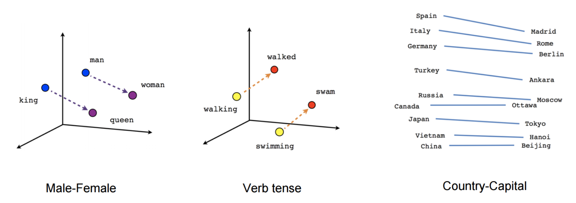
Embedding
Embedding model learns to map each discrete word into a low-dimensional continuous vector-space from their distributional properties observed in some raw text corpus.
Embedding


Embedding
Word2Vec
Premise: words next to each other are related
Two distinct models:
- CBOW (Continuous Bag of Words): given surrounding words, predict central word
- SGNS (Skip Gram with Negative Sampling): given a word, predict surrounding words
Word2Vec: SGNS
Sentence: "The quick brown fox jumps over the lazy dog"
Window = 1 Negative sample = 2
| Word | Context |
|---|---|
| the | quick |
| quick | the |
| quick | brown |
| brown | quick |
| brown | fox |
| [...] | [...] |
| Word | False Context |
|---|---|
| the | random_word1 |
| the | random_word2 |
| quick | random_word3 |
| quick | random_word4 |
| brown | random_word5 |
| [...] | [...] |
Positive Dataset D (label 1)
Negative Dataset D' (label 0)
Word2Vec: SGNS
-
Considering:
-
Corpus of words w ∈ W and their context c ∈ C
-
Parameters θ controlling the distribution P(D = 1|w, c; θ)
-
Vectorial representation of w and c:
Probability that a couple (w, c) belongs to D:
Objective:
Word2Vec: in pratice
Python library gensim: https://radimrehurek.com/gensim/models/word2vec.html
2 methods:
Usually, people use a lot of pre-trained Word2Vec models!
- Most famous: https://github.com/3Top/word2vec-api
A lot of built-in functions:
import gensim
import pandas as pd

# Method 1: Train your own model
train = pd.read_csv('train.csv', encoding="ISO-8859-1")
sentences = train[['product_title', 'search_term']].values.flatten()
model = Word2Vec(sentences, size=100, window=5, negative=5, alpha=0.025, min_count=10)

# Use a pre-trained model
# Download there: https://drive.google.com/file/d/0B7XkCwpI5KDYNlNUTTlSS21pQmM/edit
model = gensim.load_word2vec_format('GoogleNews-vectors-negative300.bin.gz')
print(model.words)  # list of words in dictionary
print(model['king'])  # get the vector of the word 'king'
Word2Vec: in pratice
model.wv.most_similar(positive=['woman', 'king'], negative=['man'])
# [('queen', 0.50882536), ...]

model.wv.doesnt_match("breakfast cereal dinner lunch".split())
# 'cereal'

model.similarity('france', 'spain')
A lot of built-in functions:
GloVe
Another embedding method:
- Word2vec is a "predictive" model
- GloVe is a "count-based" model
Count-based models:
Learn their vectors by doing some dimensionality reduction on the co-occurence counts matrix.
Always the same objective: minimize some "construction loss" when trying to find the lower-dimensional representation which can explain most of the variance in the high-dimensional data.
GloVe: quick insight
tl;dr: normalizing the counts & log-smoothing
Weighting the counts around the window:
Sentence: "word1 word2 word3 word4"
Window: 2
| word1 | word2 | word3 | word4 | |
| word1 | 0 | 1 | 0.5 | 0 |
| word2 | 1 | 0 | 1 | 0.5 |
| word3 | 0.5 | 1 | 0 | 1 |
| word4 | 0 | 0.5 | 1 | 0 |
GloVe: quick insight
Based on this matrix, vectors are built using:
Where Xij is the element (i,j) of the co-occurence matrix
Weight function g:
Cost function:
GloVe: in practice
Python library & pre-trained models:
Fast-Text
State Of the Art for word embedding
Library:
https://github.com/facebookresearch/fastText
Pre-trained models for 294 languages: https://github.com/facebookresearch/fastText/blob/master/pretrained-vectors.md
# pip install fasttext
import fasttext

import scipy
import numpy as np

model = fasttext.load_model('model.bin')
print(model.words) # list of words in dictionary
print(model['king']) # get the vector of the word 'king'

stop = []  # Stop words?

def cos_similarity(data_1, data_2):
    # Embedding for a sentence = mean of word embedding. Could it be better?
    sent1_emb = np.mean([model[x] for word in data_1 for x in word.split() if x not in stop], axis=0)
    sent2_emb = np.mean([model[x] for word in data_2 for x in word.split() if x not in stop], axis=0)

    return 1. - scipy.spatial.distance.cosine(sent1_emb, sent2_emb)
Fast-Text
whatisit
Fasttext is essentially an extension of word2vec model.
It treats each word as composed of character ngrams. So the vector for a word is made of the sum of this character n grams.
For example the word vector “apple” is a sum of the vectors of the n-grams “<ap”, “app”, ”appl”, ”apple”, ”apple>”, “ppl”, “pple”, ”pple>”, “ple”, ”ple>”, ”le>” (assuming hyperparameters for smallest ngram[minn] is 3 and largest ngram[maxn] is 6)
Fast-Text
advantages
- Rare words
- OOV words
- In theory, using character level embeddings seem to improve performances (but at a huge computational cost)
Problème : Le contexte
I like to eat my cereals with an apple.
Apple is a highly profitable company.
Le mot "Apple" est représenté par un seul vecteur dans l'espace.
Envie :
Avoir une représentation du mot "Apple" dans une région de l'espace avec de la nourriture pour la première phrase et une autre représentation dans une région avec des noms d'entreprise pour la deuxième phrase.
Optionnal:
Bert & Friends
Aller plus loin
Useful Tool:
https://projector.tensorflow.org/
T-SNE?
https://mlexplained.com/2018/09/14/paper-dissected-visualizing-data-using-t-sne-explained/
U-MAP?
https://pair-code.github.io/understanding-umap/
U-MAP > T-SNE
Min(challenge):
- Apply some cleaning & standardization for the textual data
- Build smart feature engineering based on TF-IDF (TF-IDF is a sparse vector space model for words / sentences)
- Same with at least an embedding metho : Word2Vec (gensim) is the easier; either re-use a pre-trained model or build your own w2v model