A Decision Network Design for Efficient Semantic Segmentation Computation in Edge Computing
School:National Tsing Hua University
Department: Computer Science
Student:張芸綺 Yun-Chi Chang
Advisor:李濬屹 Chun-Yi Lee
Outline
- Motivation
- Contirbution
- Background & related work
- Architecture
- Experimental results
- Conclusion
Motivation
- In recent years, deep convolutional neural networks (DCNNs) have become a popular research topic and are widely used in computer vision.
- With the grow of Internet of Things (IoT), it is more and more important to apply DCNNs to edge-end embedded devices.
Motivation
- Model distillation is often apply on classification issue, however semantic segmentation, which requires performing dense pixel-level predictions is hard to compress the model.
- The limitation of computational capabilities and power makes it hard to apply DCNN on edge-end devices.
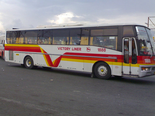

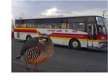
input image
prediction
bus?
car?
background?
Motivation
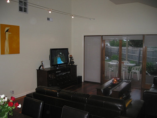
- We observed that there are some cases a simpler model can also do excellent works.
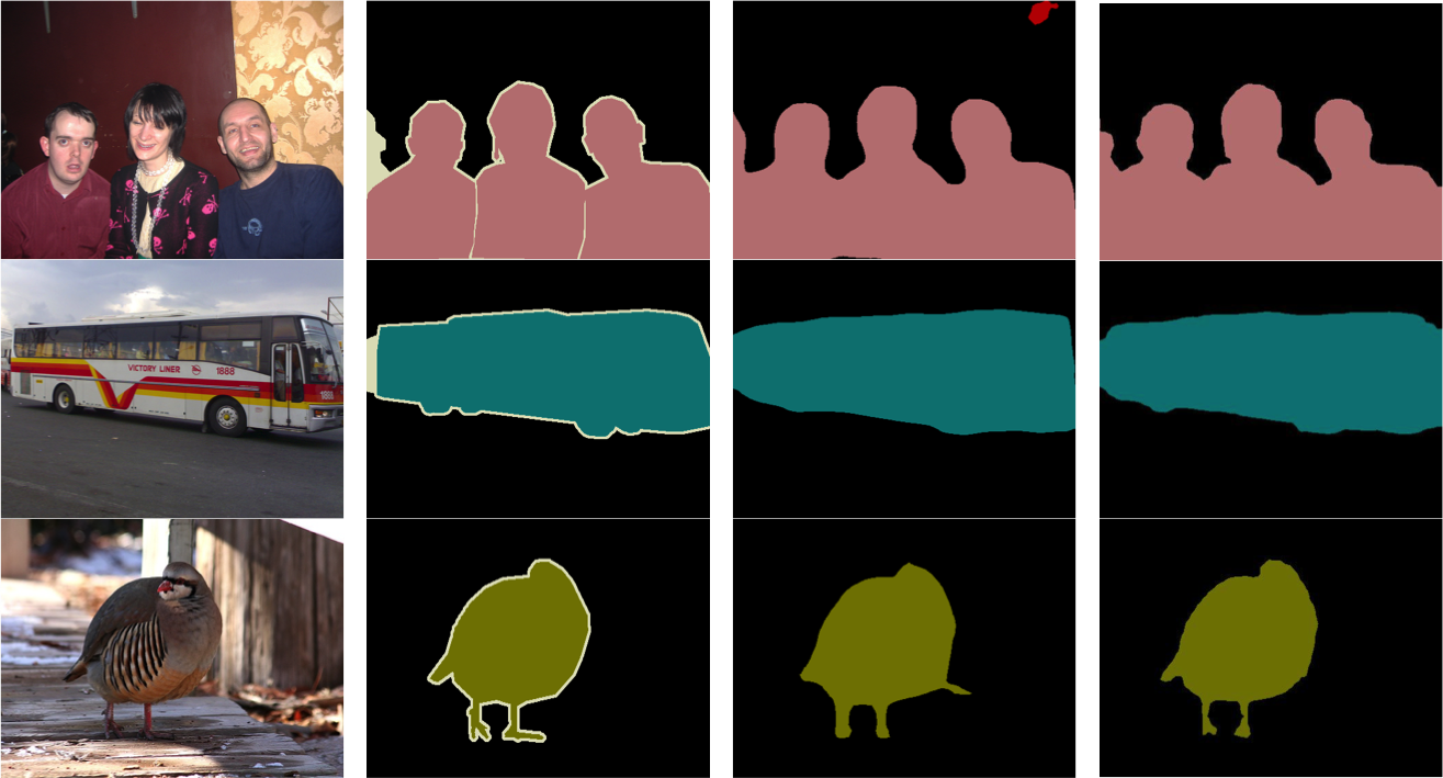
Input image
Ground truth
DeepLab-VGGNet
DeepLab-ResNet-101
Motivation
- And some get better prediction on a complicated (deeper) model.
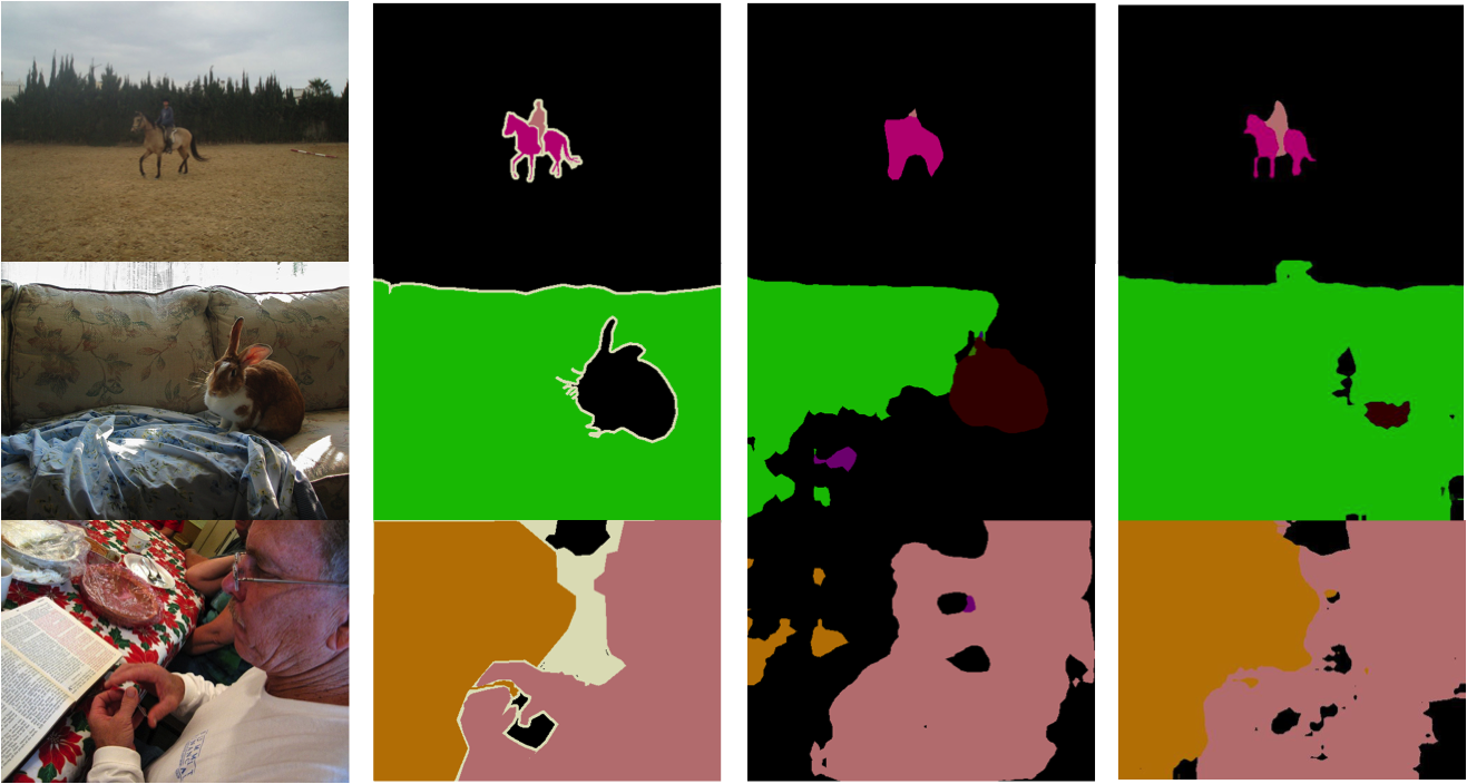
Input image
Ground truth
DeepLab-VGGNet
DeepLab-ResNet-101
Motivation
Is input image well-performed?
Yes
No
- We are aiming to train a network that classifies the input images into two categories, one for the remote, very deep model and the other for the local, lighter model.
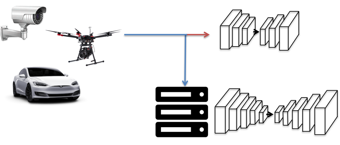
Edge-end devices
Server
Small network on edge-end devices
Large network on remote server
Contribution
- We design a Decision Network and Control Unit to predict how well the prediction of an input image will be.
- We could save overall 16.34% computation load with only 2.97% accuracy drop.
- Our Decision Network could dynamically distribute computation load base on the condition of the edge-end device.
Background & related work
- Deep convolutional neural network (DCNN)
-
DCNN on image recognition
- VGGNet
- ResNet
-
DCNN on object detection
- RCNN
- Fast-RCNN
- Faster-RCNN
-
Semantic segmentation
- FCN
- DeepLab
- Knowledge distillation
Background & related work
- Deep convolutional neural network (DCNN)
-
DCNN on image recognition
- VGGNet
- ResNet
-
DCNN on object detection
- RCNN
- Fast-RCNN
- Faster-RCNN
-
Semantic segmentation
- FCN
- DeepLab
- Knowledge distillation
Deep convolutional neural network (DCNN)
- Deep convolution neural network (DCNN) is now a popular topic and widely used in many fields like image recognition and object detection.
- DCNN does an excellent work on extracting features of images.
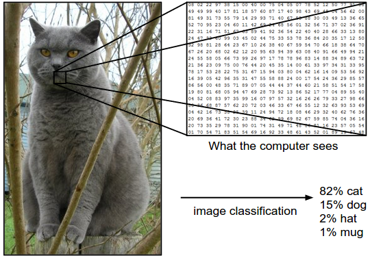
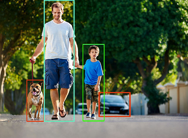
Image recognition
Object detection
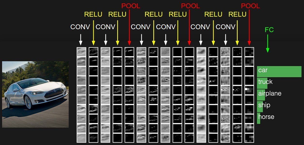
Deep convolutional neural network (DCNN)
- It is build with many convolutional layers, activation functions and pooling layers.
Background & related work
- Deep convolutional neural network (DCNN)
-
DCNN on image recognition
- VGGNet
- ResNet
-
DCNN on object detection
- RCNN
- Fast-RCNN
- Faster-RCNN
-
Semantic segmentation
- FCN
- DeepLab
- Knowledge distillation
DCNN on Image Recognition
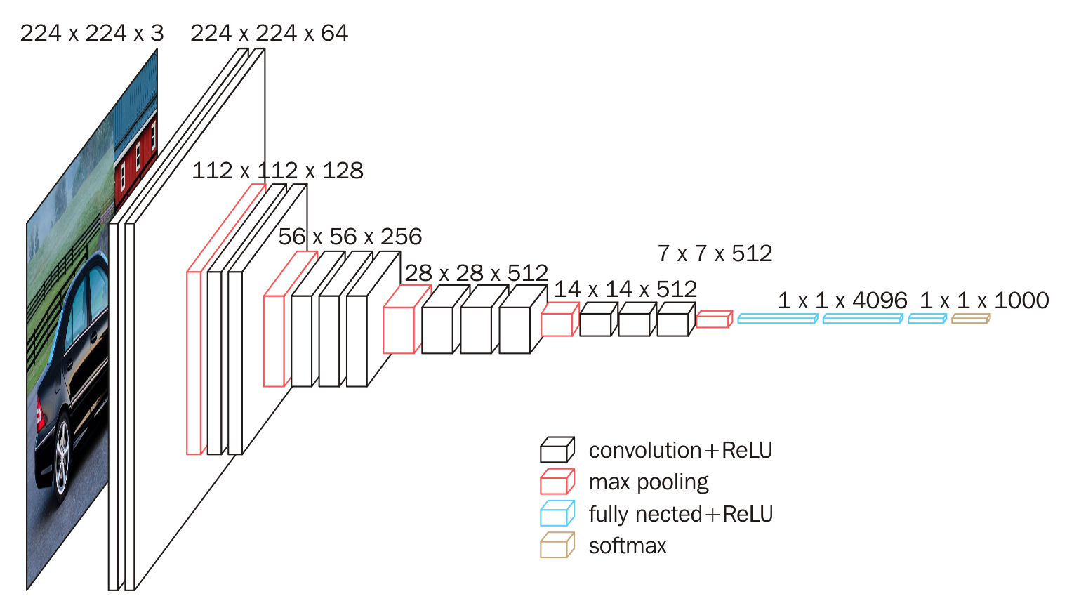
- Numbers of researches on image recognition are designed base on a very deep CNN.
- VGGNet is one of representative work, which consist of 5 convolutional groups, and 3 FC layers.
DCNN on Image Recognition
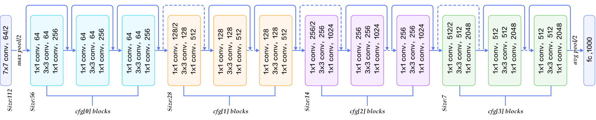
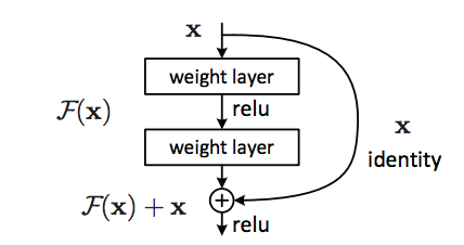
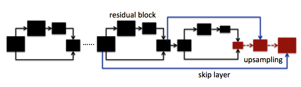
- ResNet is one of the outstanding works on image recognition, it is build by blocks that could be flexibly extended.
Background & related work
- Deep convolutional neural network (DCNN)
-
DCNN on image recognition
- VGGNet
- ResNet
-
DCNN on object detection
- RCNN
- Fast-RCNN
- Faster-RCNN
-
Semantic segmentation
- FCN
- DeepLab
- Knowledge distillation
DCNN on object detection
- There are two main methods for detecting objects: bounding box and semantic segmentation.
- Bounding box method predicts the location and the borders of objects using boxes.
Bounding Box
DCNN on object detection
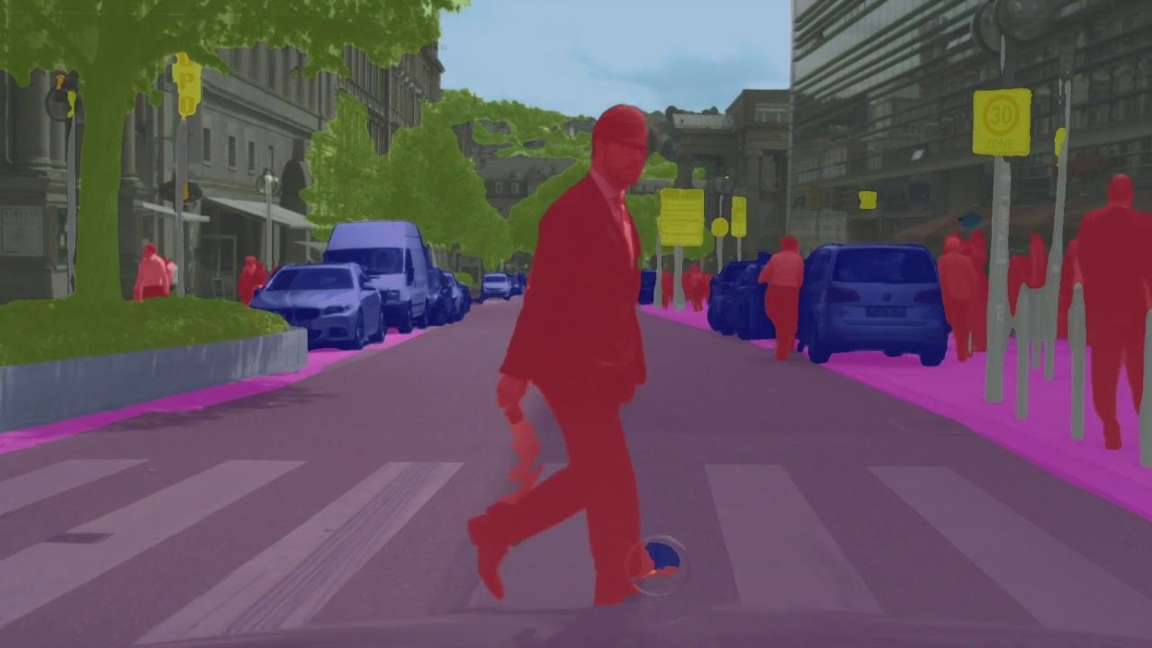
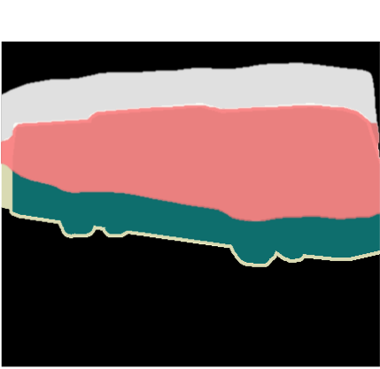
- Semantic segmentation mask out the objects using pixel-wise prediction.
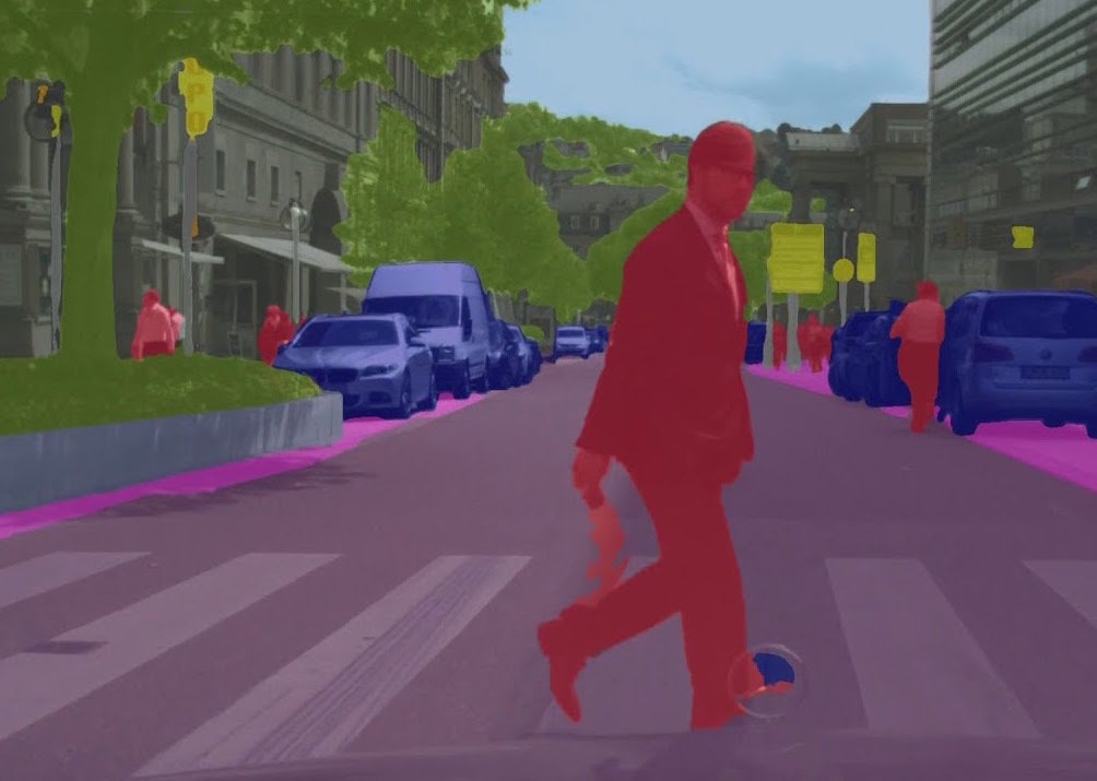
Semantic Segmentation
Region-based Convolutional Neural Networks (R-CNN)
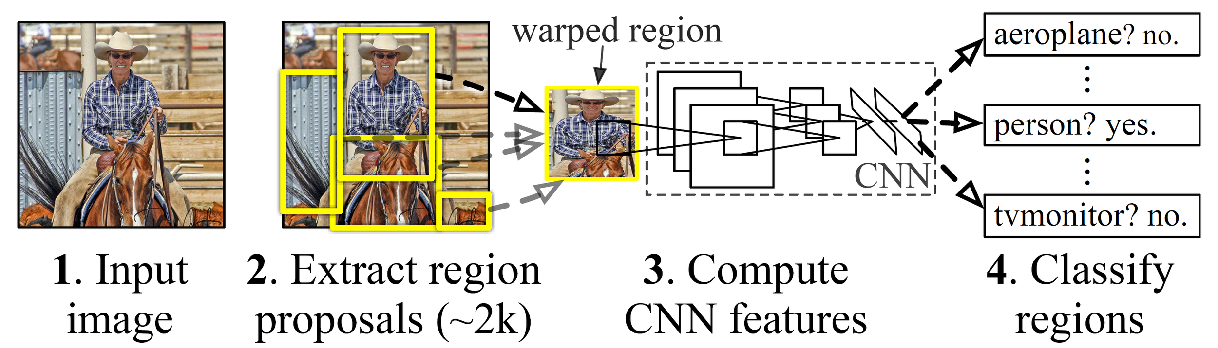
- Use selective selection to extract over 2,000 region proposals. (slow)
- Each region proposal computes CNN.
- Many region proposals are overlapping, therefore RCNN is not efficient.
- Drawbacks: slow and inefficient
- Fast-RCNN extracts features of region proposals after the whole image goes through CNN.
- A common CNN is used for feature extraction.
- Drawback: Region proposal extraction is still time-consuming
RCNN Fast-RCNN
Fast R-CNN
Faster-RCNN

- Faster-RCNN use Region Proposal Network (RPN) to predict region proposals instead of selective search.
Background & related work
- Deep convolutional neural network (DCNN)
-
DCNN on image recognition
- VGGNet
- ResNet
-
DCNN on object detection
- RCNN
- Fast-RCNN
- Faster-RCNN
-
Semantic segmentation
- FCN
- DeepLab
- Knowledge distillation
Semantic Segmentation
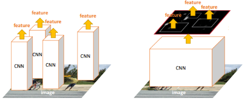
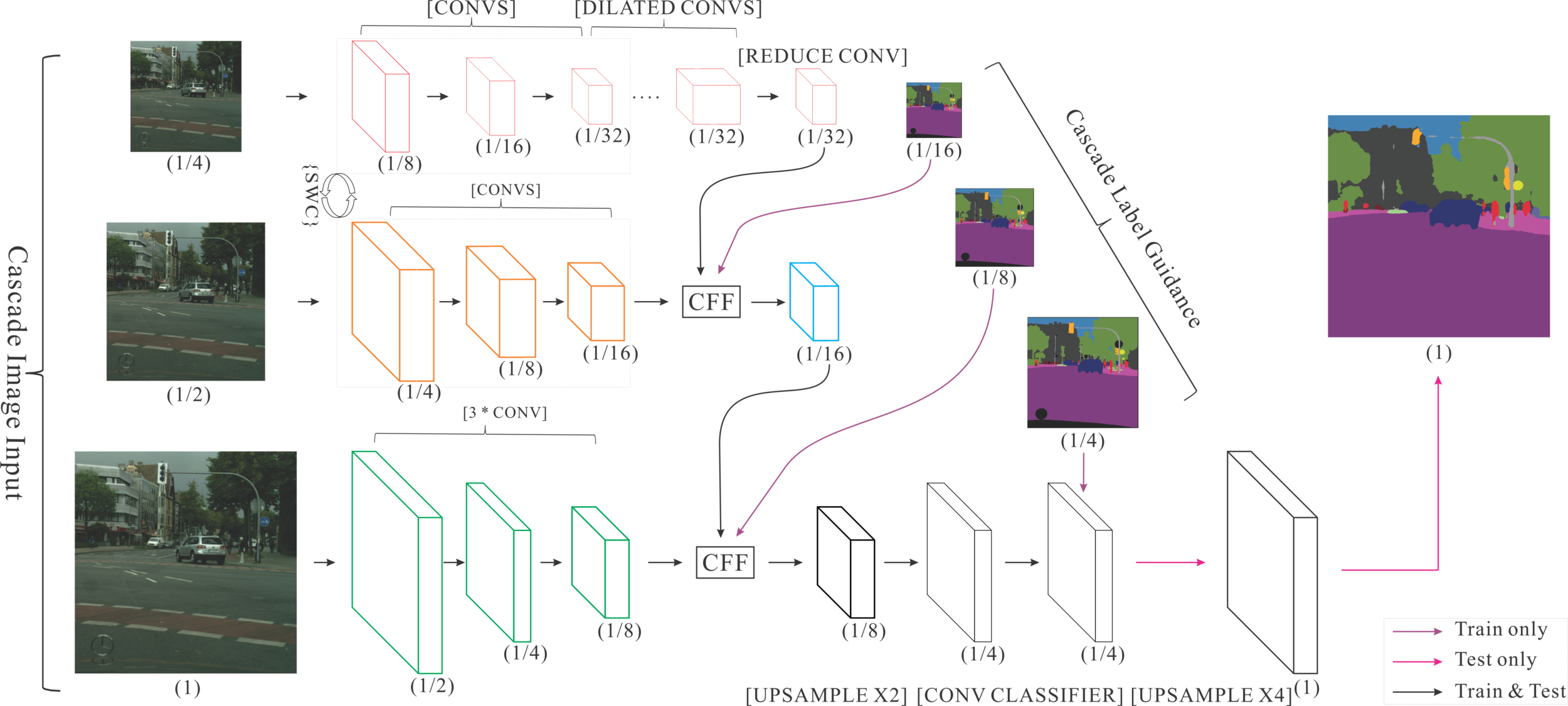
- Semantic segmentation methods are expected to output pixel-wise prediction, so that the resolution of the output feature maps becomes very important.
Semantic Segmentation
-
There are lots of methods focusing on keeping the high resolution of features.
- multi-scale inputs
- skip-architecture
- atrous convolution
- We often use mIoU to measure the accuracy of our segmentation prediction.
- The mIoU is defined as mean of IoUs.
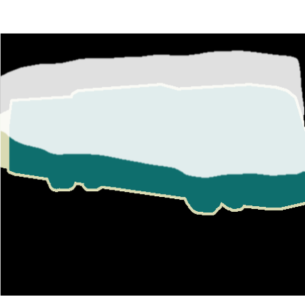
Union of the prediction and the ground truth
Overlap of the prediction and the ground truth
Semantic Segmentation
: Number of objects in the data set.
- We often use mIoU to measure the accuracy of our segmentation prediction.
- The mIoU is defined as mean of IoUs.
Union of the prediction and the ground truth
Overlap of the prediction and the ground truth
Semantic Segmentation
: Number of objects in the data set.
- FCN replaced all fully-connected layers by convolutional layers and accept arbitrary-sized input.
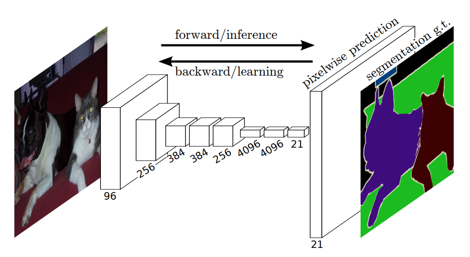
FCN
- Skip-architecture
- Early layers contain higher resolution features which preserve more localization information.
- Ending layers in the deep path contain more context information.
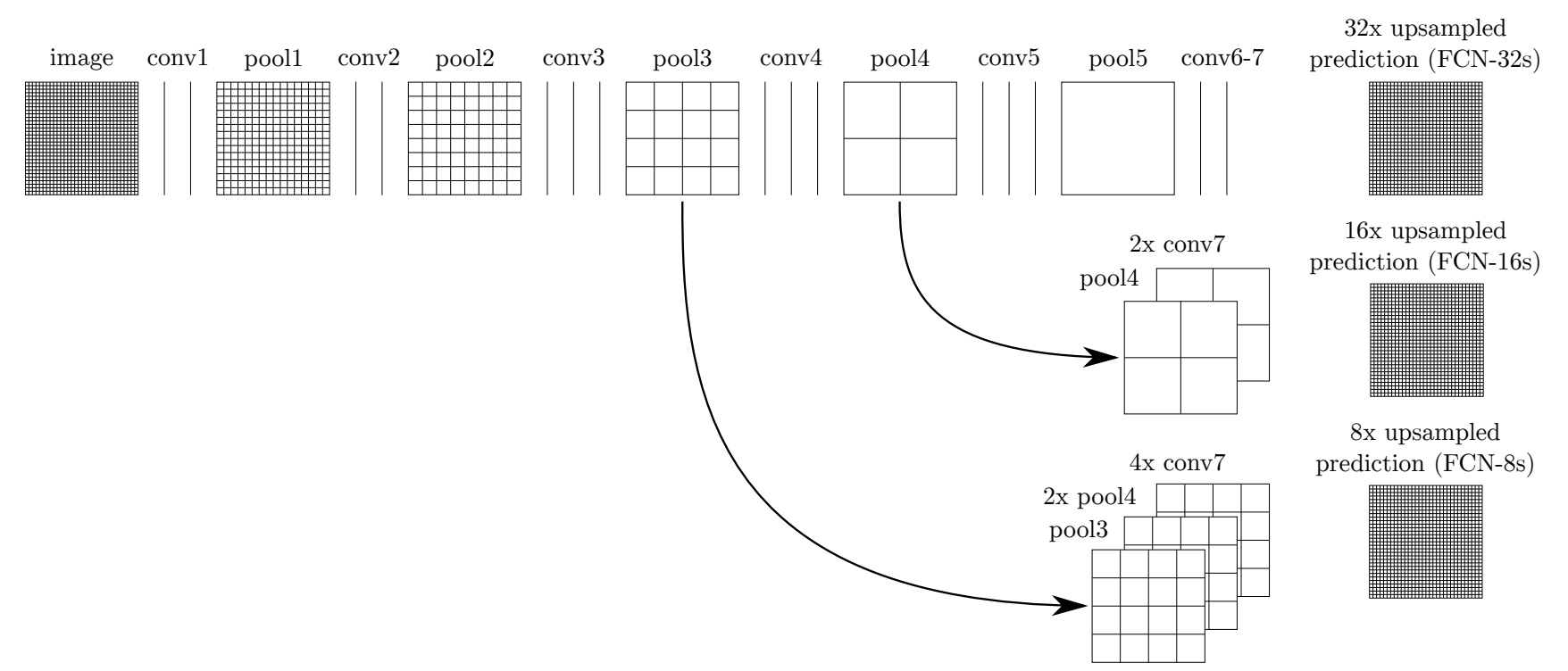
FCN
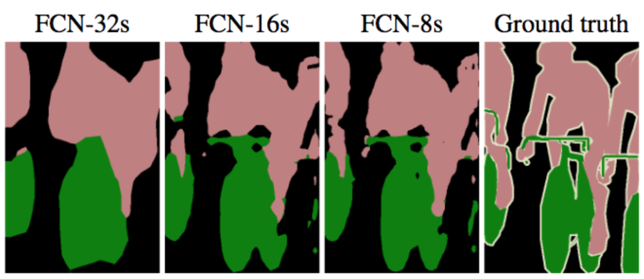
FCN
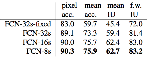
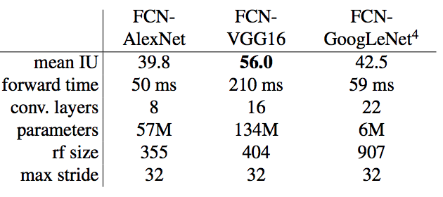
-
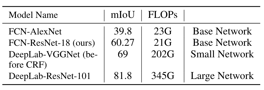
FCN-AlexNet
- lightest semantic segmentation model
- we fine-tune it in our work
- mIoU is only 39.8%
FCN
DeepLab
- DeepLab-v2 claims an excellent result on semantic segmentation.
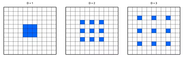
- Atrous convolution is applied.

DeepLab
- Replace pooling layer and keep the resolusion.
- No extra overhead (weight) is needed for the atrous convolution.
DeepLab
- Replace pooling layer and keep the resolusion.
- No extra overhead (weight) is needed for the atrous convolution.
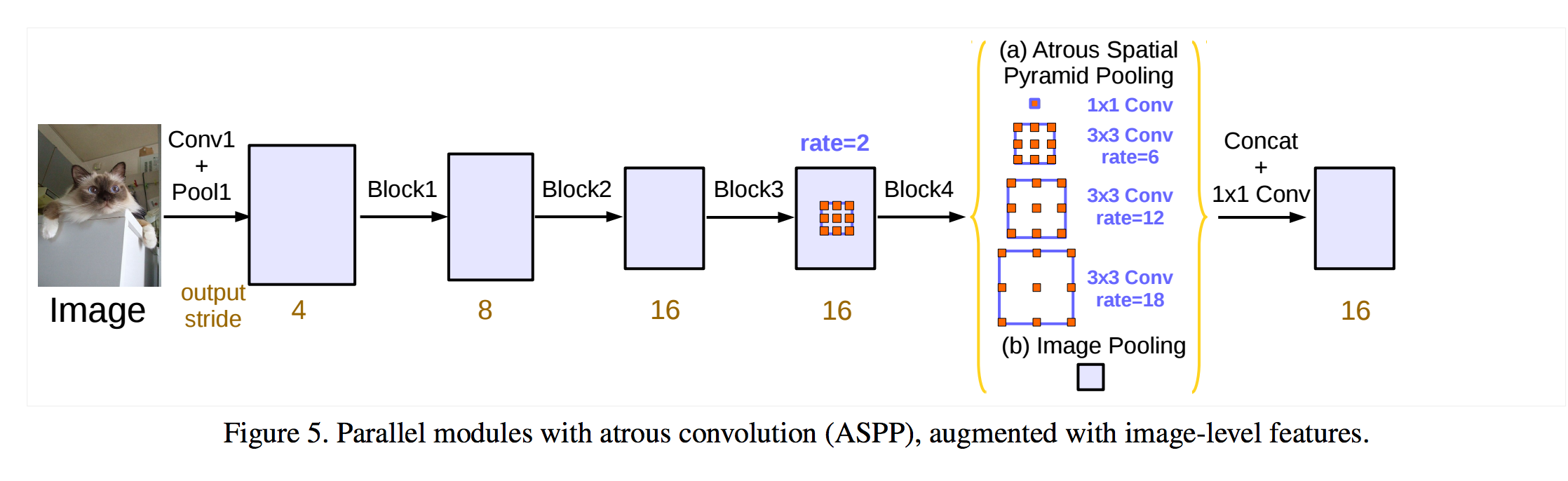
DeepLab
DeepLab-v3 add an image pooling layer in ASPP.
- Replace pooling layer and keep the resolusion.
- No extra overhead (weight) is needed for the atrous convolution.
Background & related work
- Deep convolutional neural network (DCNN)
- DCNN on classification
- VGGNet
- ResNet
- DCNN on object detection
- RCNN
- Fast-RCNN
- Faster-RCNN
- Semantic segmentation
- FCN
- DeepLab
- Knowledge distillation
Knowledge distillation
- The main concept is training a smaller model "student" to imitate the behavior of the original model "teacher".
- The teacher provides its prediction as the label for the student model so the student gets more information.
Knowledge distillation
- Most model distillation works only deal with classification problems.
- It is due to the requirement for much more high-dimensional information from an image to perform dense predictions at pixel level.
Architecture
- Architecture Introduction
- Decision Network
- Architecture
- Base Network
- SPP Layer
- IoU prediction
- Training Methodology
- The Control Unit
Architecture Introduction
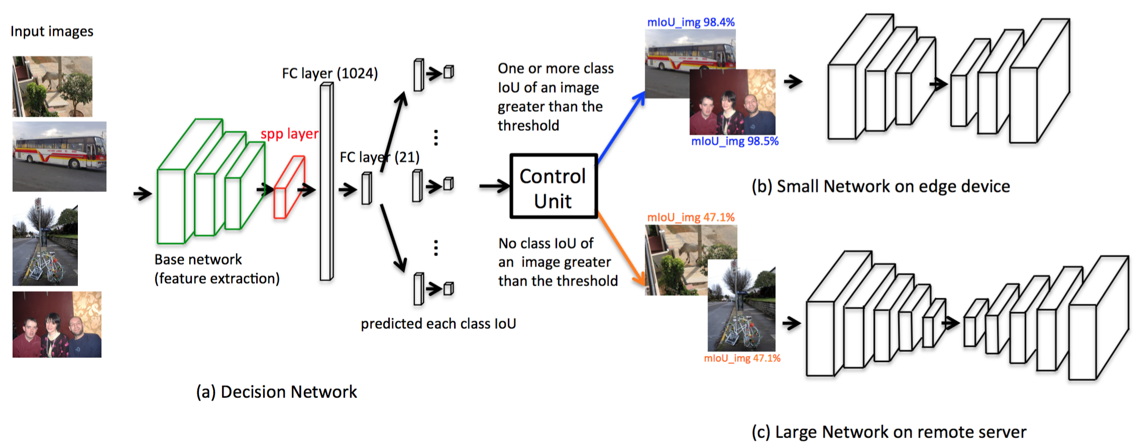
The architecture of our work contains four parts:
- Decision Network
- Control Unit
- Small Network
- Large Network
-
Our Decision Network:
- It is trained for predicting the IoU of each class.
-
The Control Unit:
- Assign some well-performed images to the remote server and adjust the computation load of the local device.
Architecture Introduction
- The small network evaluate images at the embedded end.
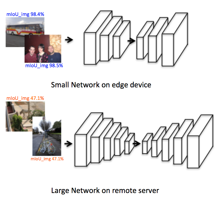
- Reduce computation at the edge-end and get a close result to the large network's.
Architecture Introduction
DeepLab-VGGNet (mIoU=69%)
DeepLab-ResNet-101 (mIoU=81%)
- The large network runs at the server end
Our Goal
DeepLab-VGGNet
DeepLab-ResNet-101
Architecture
- Architecture Introduction
-
Decision Network
- Architecture
- Base Network
- SPP Layer
- IoU prediction
- Training Methodology
- The Control Unit
Decision Network - Architecture
The Decision Network contains:
- Base network
- SPP layer
- Two shared fully-connected layer with 1,024 and 21 channels
- One small 21-channel-fully-connected layer for each class
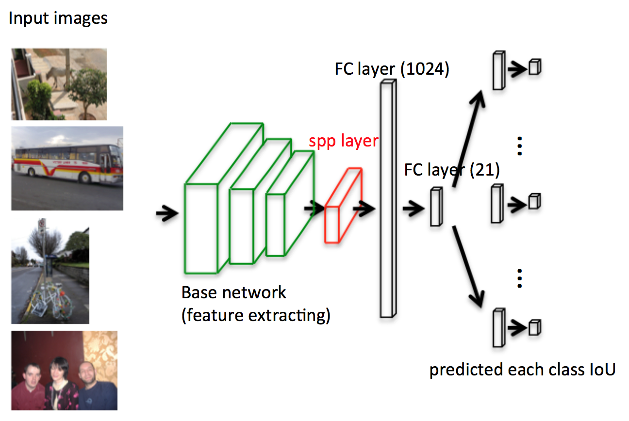
(feature extraction)
Decision Network - Base Network
- We use pre-trained FCN-AlexNet as the base feature extraction network of Decision-Network-AlexNet.
- We fixed the parameters of the base network during training to keep the ability of feature extraction.
Decision Network - Base Network
- We also trained another base network FCN-ResNet-18 for Decision-Network-ResNet-18, which is a combination of the skip-architecture and ResNet-18.
- Our FCN-ResNet-18 reaches an mIoU of 60.27% on VOC 2012 validation set, which is 20.47% higher than FCN-AlexNet (39.8%).
The Decision Network contains:
- Base network
- SPP layer
- Two shared fully-connected layer with 1,024 and 21 channels
- One small 21-channel-fully-connected layer for each class
Decision Network - SPP Layer
(feature extraction)
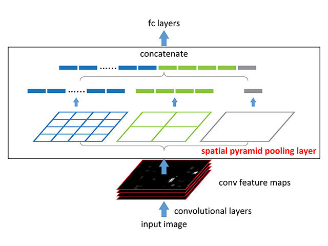
- To keep the whole view of the image, we have to make sure the network is flexible and accepts arbitrary-sized input.
Decision Network - SPP Layer
- To keep the whole view of the image, we have to make sure the network is flexible and accepts arbitrary-sized input.
- We add a two-layer-tall spacial pyramid pooling layer (SPP) after the fixed base network to fit the fixed-length vector from different size of feature map.
Decision Network - SPP Layer
The mIoU is defined as:
Decision Network - IoU Prediction
We define IoU_img to estimate our accuracy on an image:
: Number of classes contained in an image
: Number of objects in the data set.
Decision Network - IoU Prediction
- We use DeepLab-VGGNet to generate the ground truth vector of each class IoU.
0 0 0.95 0 0 0 0 0 0 0 0 0 0 0 0 0 0 0 0 0
0 0 0.95 0 0 0.98 0 0 0 0 0 0 0 0 0 0 0 0 0 0
IoU_img = 0.95 / 1 = 0.95
IoU_img = (0.95 + 0.98) / 2
= 0.965
- well-performed image is defined as IoU_img > 0.7
- The distribution of IoU_img is concentrate to more than 70%.
- The distribution of each class IoU is well-distributed in non-zero cases.
Decision Network - IoU Prediction
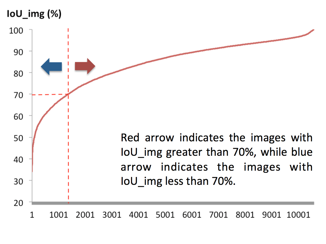
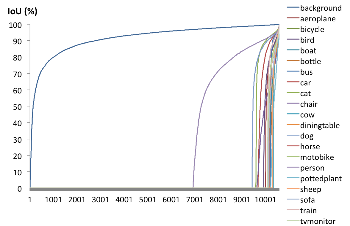
Image number
Image number
Decision Network - IoU Prediction
- The distribution of IoU_img is concentrate to more than 70%.
- The distribution of each class IoU is well-distributed in non-zero cases.
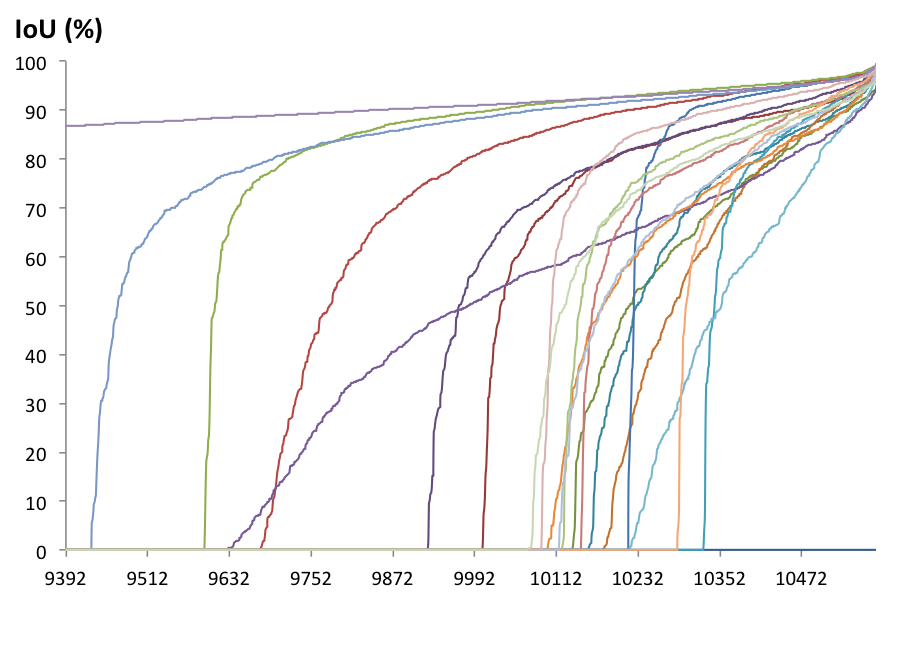
Image number
Image number
Decision Network - IoU Prediction
- The higher score we get, the higher chance will the image be well-performed on the small network.
- The prediction IoU of each class is bounded to [0,1].
- ground truth people IoU: 0.9548
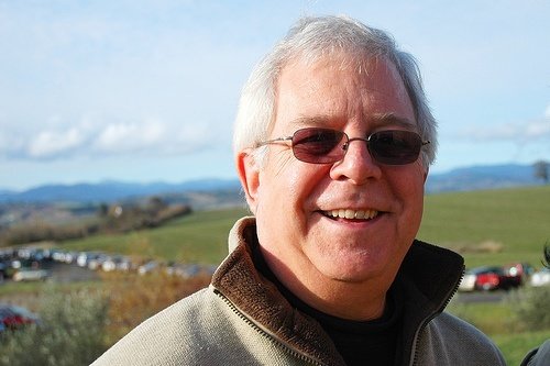
- predicted people IoU: 0.9677

Decision Network - Training Methodology
- For training strategy, we use "poly" learning rate (lr) policy mentioned in DeepLab.
- We set = 60,000, = 0.001, and = 0.9 with batch size of 20 images.
Architecture
- Architecture Introduction
- Decision Network
- Architecture
- Base Network
- SPP Layer
- IoU prediction
- Training Methodology
- The Control Unit
Decision Network - The Control Unit
- The Control Unit (CU) will decide whether an image is well-performed by checking if there are one or more class IoU is greater than the threshold.
- The threshold could be dynamically changed based on the condition of the edge-end device (battery, computation load, etc.).
CU
Experimental Results
- Experimental Setup
- Evaluation Criteria
- Experiments on Decision Network
- Computation Reduction
- Decision Network Variants
- The Control Unit
Experimental Results
- Experimental Setup
- Evaluation Criteria
- Experiments on Decision Network
- Computation Reduction
- Decision Network Variants
- The Control Unit
Experimental setup
- PASCAL VOC2012
- 10,852 labeled images
- 20 classes
- DeepLab-VGGNet as the small network
- DeepLab-ResNet-101 as the large network
Experimental Results
- Experimental Setup
- Evaluation Criteria
- Experiments on Decision Network
- Computation Reduction
- Decision Network Variants
- The Control Unit
Evaluation Criteria
To evaluate our decision network, we calculate :
true positive
false positive
- ground truth IoU_img: 0.9548
- predicted as well-performed image
- ground truth IoU_img: 0.5646
- predicted as well-performed image
Evaluation Criteria
To evaluate our decision network, we calculate :
true positive/ total images in the subset of images with IoU_img .
true negative/ total images in the subset of images with IoU_img .
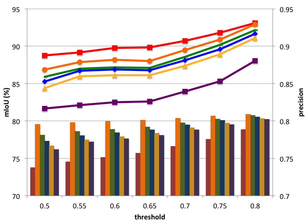
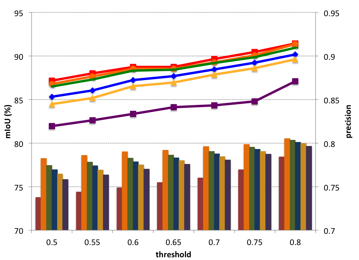
Evaluation Criteria
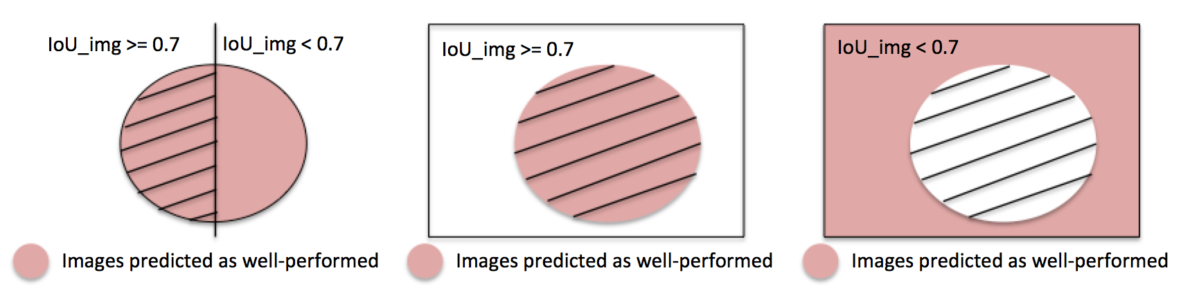
Evaluation Criteria
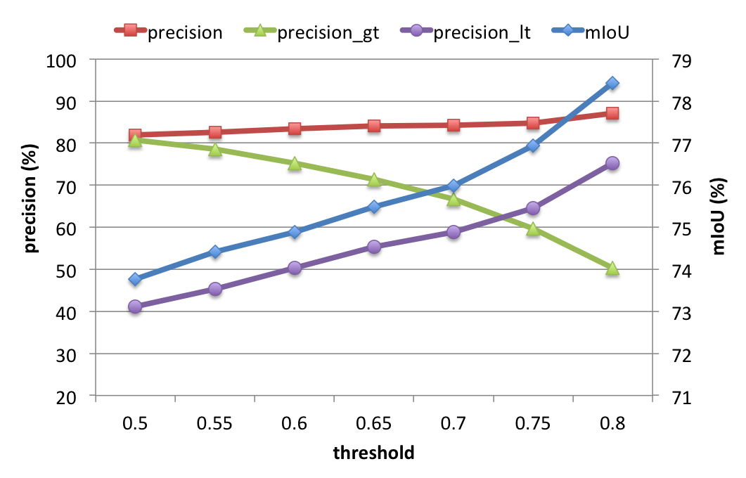
- The higher precision we get, the lower is.
Evaluation Criteria
- But the higher precision we get, the higher is.
Experimental Results
- Experimental Setup
- Evaluation Criteria
- Experiments on Decision Network
- Computation Reduction
- Decision Network Variants
- The Control Unit
Experiments on Decision Network
-
DeepLab-ResNet-101
- mIoU=81.8%
- 345G FLOPs
-
DeepLab-VGGNet
- 202G FLOPs (60% of DeepLab-ResNet-101's)
- mIoU=69%.
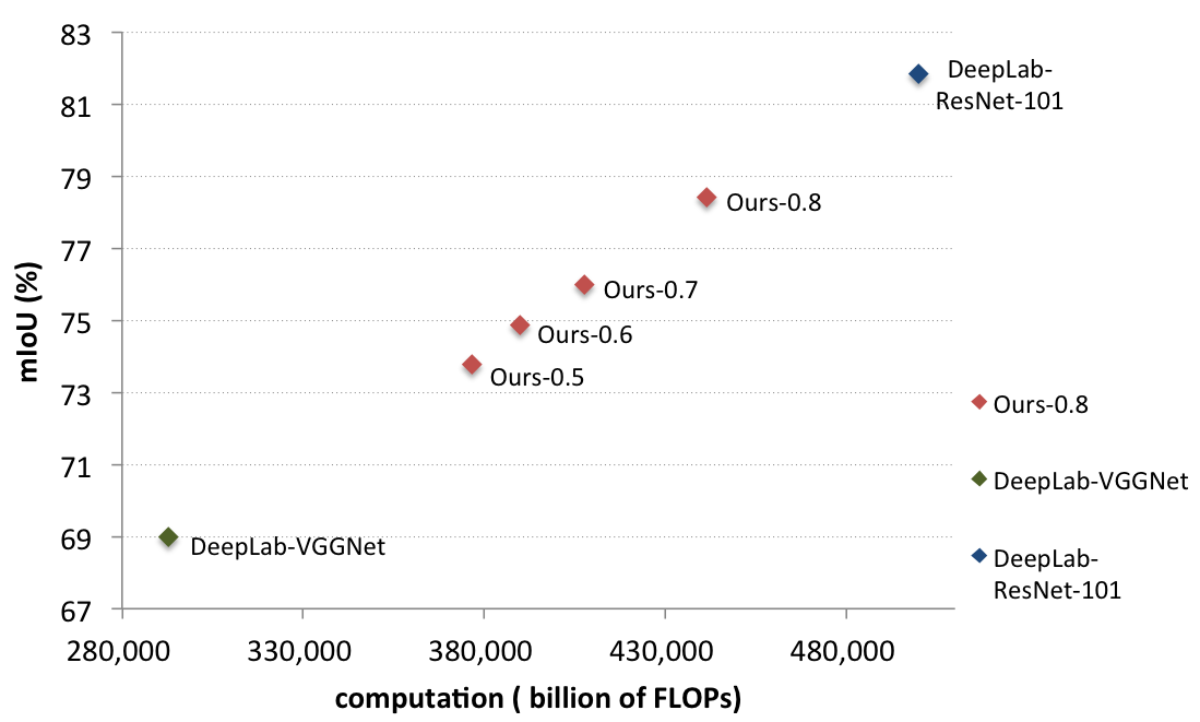
-
Our work (Decision-Network-AlexNet) reaches
- mIoU at most 78.42%
- at least 259G FLOPs is needed
Experimental Results
- Experimental Setup
- Evaluation Criteria
- Experiments on Decision Network
- Computation Reduction
- Decision Network Variants
- The Control Unit
Computation Reduction
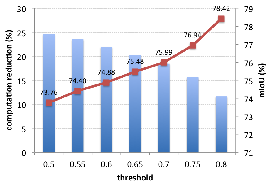
Overall computation reduction (Decision-Network-AlexNet)
- The total reduction gets lower when the threshold increases.
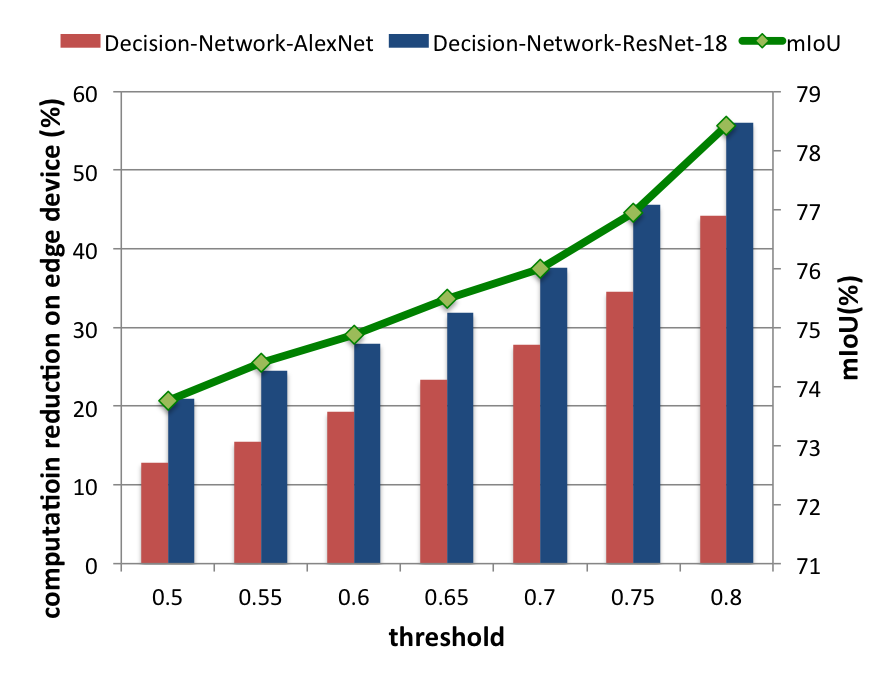
Computation Reduction
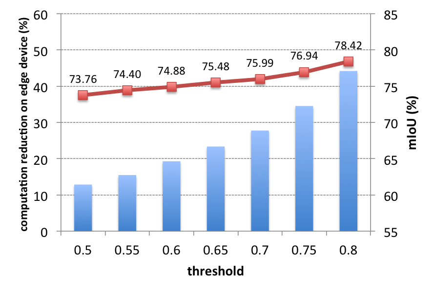
Edge-end computation reduction (Decision-Network-AlexNet)
- The reduction on edge-end gets higher when the threshold increases.
Experimental Results
- Experimental Setup
- Evaluation Criteria
- Experiments on Decision Network
- Computation Reduction
- Decision Network Variants
- The Control Unit
Decision Network Variants
-
Total computation reduction (Decision-Network-ResNet-18)
- 16.17% computation of Decision-Network-AlexNet
- 9.58% higher computation reduction in average than Decision-Network-AlexNet.
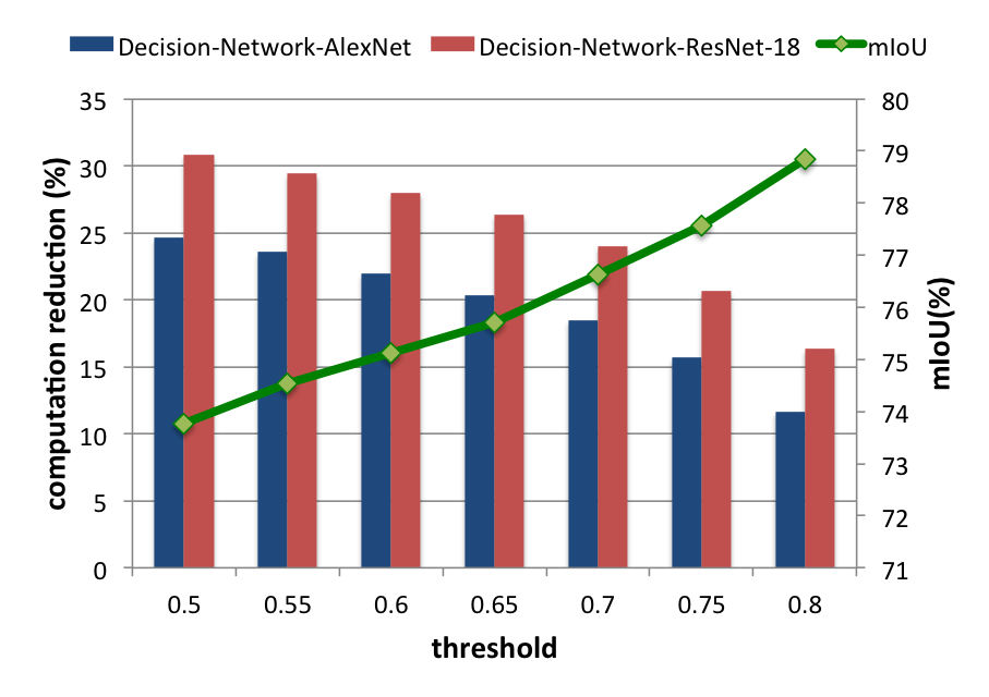
Decision Network Variants
- It is proved that we could replace our base network as any feature extracting based network.
Experimental Results
- Experimental Setup
- Evaluation Criteria
- Experiments on Decision Network
- Computation Reduction
- Decision Network Variants
- The Control Unit
The Control Unit
Decision-Network-AlexNet
Decision-Network-ResNet-101
Conclusion
- We could dynamically change our threshold to tune the computational work load on the edge-end.
- The base network can be replaced by any other feature extracting network.
- We could save at most 56.05% computation on the edge-end with only 8.04% mIoU drop.
- On average, 25.09% total computation is saved with Decision-Network-ResNet-18.
- The mIoU reaches 78.8% in our work with only 3% less than the large network DeepLab-ResNet-101.