Safety and Efficiency for Autonomous Vehicles through Online Learning
Zachary Sunberg
Current: Postdoctoral Scholar, University of California
Future: Assistant Professor, University of Colorado
How do we deploy autonomy with confidence?
Safety and Efficiency through Online Learning

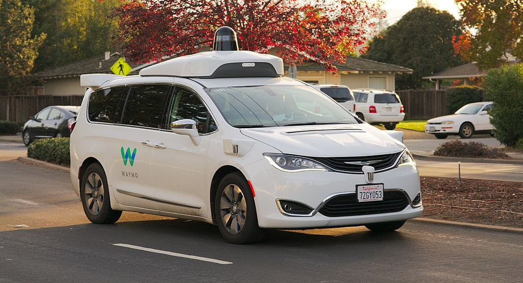
Waymo Image By Dllu - Own work, CC BY-SA 4.0, https://commons.wikimedia.org/w/index.php?curid=64517567


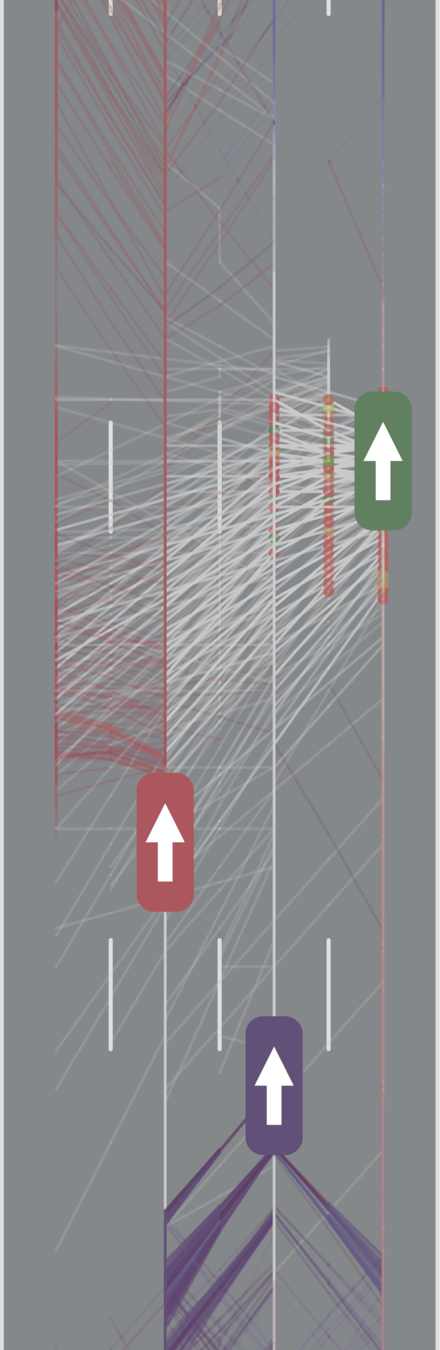
Driving
POMCPOW
POMDPs.jl

Future
POMDPs
Driving
POMCPOW
POMDPs.jl
Future
POMDPs
Tweet by Nitin Gupta
29 April 2018
https://twitter.com/nitguptaa/status/990683818825736192
Two Objectives for Autonomy
EFFICIENCY
SAFETY
Minimize resource use
(especially time)
Minimize the risk of harm to oneself and others

Safety often opposes Efficiency
Pareto Optimization
Safety
Better Performance
Model \(M_2\), Algorithm \(A_2\)
Model \(M_1\), Algorithm \(A_1\)
Efficiency
$$\underset{\pi}{\mathop{\text{maximize}}} \, V^\pi = V^\pi_\text{E} + \lambda V^\pi_\text{S}$$
Safety
Weight
Efficiency

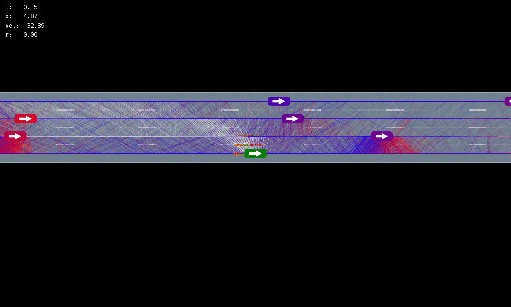
Intelligent Driver Model (IDM)
\ddot{x}_\text{IDM} = a \left[ 1 - \left( \frac{\dot{x}}{\dot{x}_0} \right)^{\delta} - \left(\frac{g^*(\dot{x}, \Delta \dot{x})}{g}\right)^2 \right]
g^*(\dot{x}, \Delta \dot{x}) = g_0 + T \dot{x} + \frac{\dot{x}\Delta \dot{x}}{2 \sqrt{a b}}

[Treiber, et al., 2000] [Kesting, et al., 2007] [Kesting, et al., 2009]
Internal States


All drivers normal


No learning (MDP)
Omniscient
POMCPOW (Ours)
Simulation results
[Sunberg, 2017]


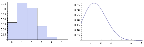
Marginal Distribution: Uniform
\(\rho=0\)
\(\rho=1\)
\(\rho=0.75\)
Internal parameter distributions
Conditional Distribution: Copula
Assume normal


No Learning (MDP)
Omniscient
Mean MPC
QMDP
POMCPOW (Ours)


[Sunberg, 2017]
Driving
POMCPOW
POMDPs.jl
Future
POMDPs
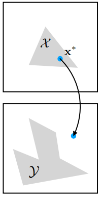
Types of Uncertainty
OUTCOME
MODEL
STATE


Markov Model
- \(\mathcal{S}\) - State space
- \(T:\mathcal{S}\times\mathcal{S} \to \mathbb{R}\) - Transition probability distributions
Markov Decision Process (MDP)
- \(\mathcal{S}\) - State space
- \(T:\mathcal{S}\times \mathcal{A} \times\mathcal{S} \to \mathbb{R}\) - Transition probability distribution
- \(\mathcal{A}\) - Action space
- \(R:\mathcal{S}\times \mathcal{A} \to \mathbb{R}\) - Reward

Solving MDPs - The Value Function
$$V^*(s) = \underset{a\in\mathcal{A}}{\max} \left\{R(s, a) + \gamma E\Big[V^*\left(s_{t+1}\right) \mid s_t=s, a_t=a\Big]\right\}$$
Involves all future time
Involves only \(t\) and \(t+1\)
$$\underset{\pi:\, \mathcal{S}\to\mathcal{A}}{\mathop{\text{maximize}}} \, V^\pi(s) = E\left[\sum_{t=0}^{\infty} \gamma^t R(s_t, \pi(s_t)) \bigm| s_0 = s \right]$$
$$Q(s,a) = R(s, a) + \gamma E\Big[V^* (s_{t+1}) \mid s_t = s, a_t=a\Big]$$
Value = expected sum of future rewards
Online Decision Process Tree Approaches

Time
Estimate \(Q(s, a)\) based on children
$$Q(s,a) = R(s, a) + \gamma E\Big[V^* (s_{t+1}) \mid s_t = s, a_t=a\Big]$$
\[V(s) = \max_a Q(s,a)\]
Partially Observable Markov Decision Process (POMDP)

- \(\mathcal{S}\) - State space
- \(T:\mathcal{S}\times \mathcal{A} \times\mathcal{S} \to \mathbb{R}\) - Transition probability distribution
- \(\mathcal{A}\) - Action space
- \(R:\mathcal{S}\times \mathcal{A} \to \mathbb{R}\) - Reward
- \(\mathcal{O}\) - Observation space
- \(Z:\mathcal{S} \times \mathcal{A}\times \mathcal{S} \times \mathcal{O} \to \mathbb{R}\) - Observation probability distribution
\begin{aligned}
& \mathcal{S} = \mathbb{Z} \quad \quad \quad ~~ \mathcal{O} = \mathbb{R} \\
& s' = s+a \quad \quad o \sim \mathcal{N}(s, s-10) \\
& \mathcal{A} = \{-10, -1, 0, 1, 10\} \\
& R(s, a) = \begin{cases}
100 & \text{ if } a = 0, s = 0 \\
-100 & \text{ if } a = 0, s \neq 0 \\
-1 & \text{ otherwise}
\end{cases} & \\
\end{aligned}

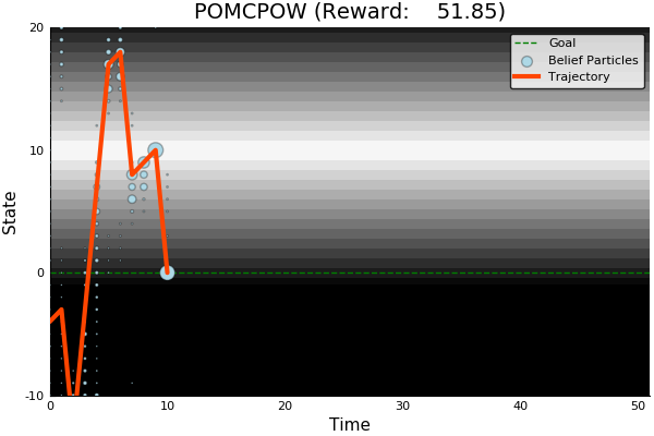
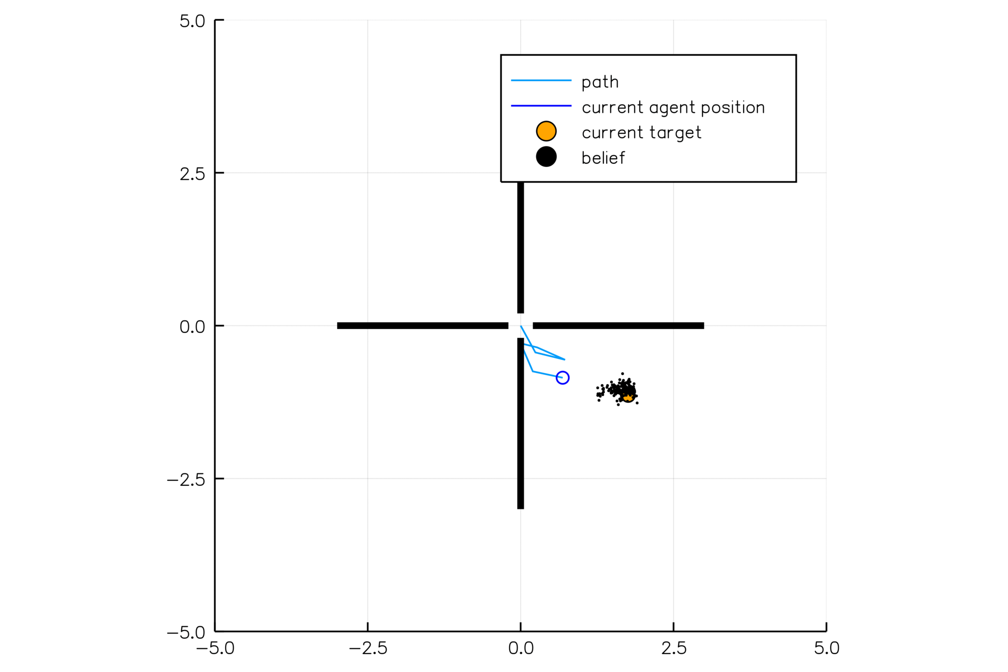
State
Timestep
Accurate Observations
Goal: \(a=0\) at \(s=0\)
Optimal Policy
Localize
\(a=0\)
POMDP Example: Light-Dark
POMDP Sense-Plan-Act Loop
Environment
Belief Updater
Policy
\(b\)
\(a\)
\[b_t(s) = P\left(s_t = s \mid a_1, o_1 \ldots a_{t-1}, o_{t-1}\right)\]

True State
\(s = 7\)
Observation \(o = -0.21\)
Environment
Belief Updater
Policy
\(a\)
\(b = \mathcal{N}(\hat{s}, \Sigma)\)
True State
\(s \in \mathbb{R}^n\)
Observation \(o \sim \mathcal{N}(C s, V)\)
LQG Problem (a simple POMDP)
\(s_{t+1} \sim \mathcal{N}(A s_t + B a_t, W)\)
\(\pi(b) = K \hat{s}\)
Kalman Filter
\(R(s, a) = - s^T Q s - a^T R a\)
Real World POMDPs


1) ACAS
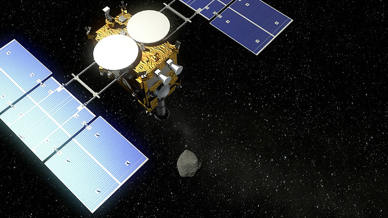
2) Orbital Object Tracking
4) Medical
3) Dual Control
ACAS X
Trusted UAV
Collision Avoidance
[Sunberg, 2016]
[Kochenderfer, 2011]
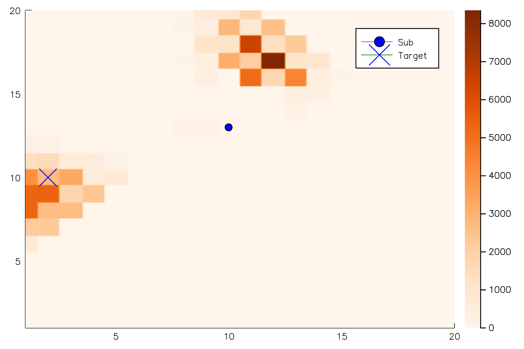
Real World POMDPs
\(\mathcal{S}\): Information space for all objects
\(\mathcal{A}\): Which objects to measure
\(R\): - Entropy
Approximately 20,000 objects >10cm in orbit
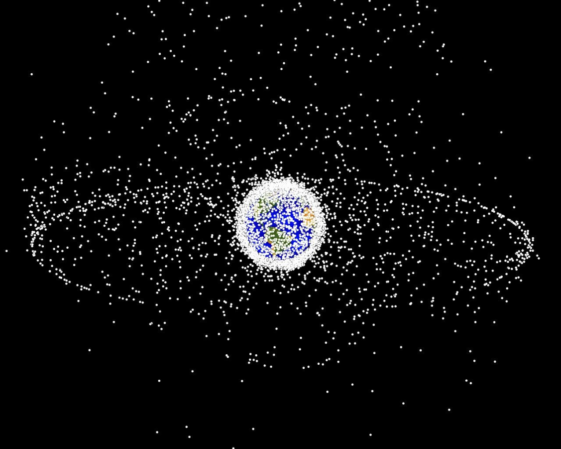
[Sunberg, 2016]
1) ACAS
2) Orbital Object Tracking
4) Medical
3) Dual Control
Real World POMDPs


State \(x\) Parameters \(\theta\)
\(s = (x, \theta)\) \(o = x + v\)
POMDP solution automatically balances exploration and exploitation
[Slade, Sunberg, et al. 2017]
1) ACAS
2) Orbital Object Tracking
4) Medical
3) Dual Control
Real World POMDPs
1) ACAS
2) Orbital Object Tracking
4) Medical
3) Dual Control
[Ayer 2012]

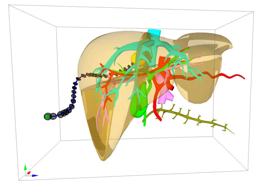
[Sun 2014]
Personalized Cancer Screening
Steerable Needle Guidance
Driving
POMCPOW
POMDPs.jl
Future
POMDPs
POMDP Sense-Plan-Act Loop
Environment
Belief Updater
Policy

\(o\)
\(b\)
\(a\)
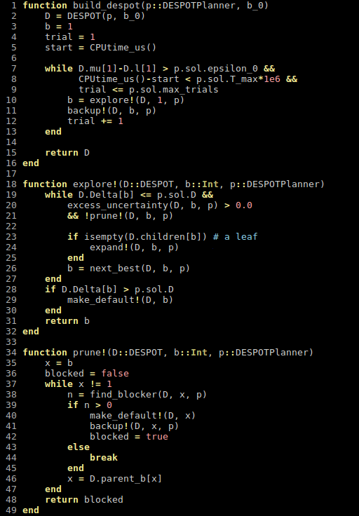
- A POMDP is an MDP on the Belief Space but belief updates are expensive
- POMCP* uses simulations of histories instead of full belief updates
- Each belief is implicitly represented by a collection of unweighted particles

[Ross, 2008] [Silver, 2010]
*(Partially Observable Monte Carlo Planning)
[ ] An infinite number of child nodes must be visited
[ ] Each node must be visited an infinite number of times
Solving continuous POMDPs - POMCP fails

POMCP
✔
✔
Double Progressive Widening (DPW): Gradually grow the tree by limiting the number of children to \(k N^\alpha\)
Necessary Conditions for Consistency
[Coutoux, 2011]

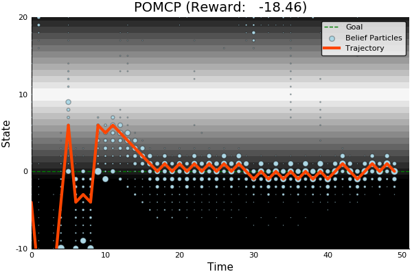
POMCP
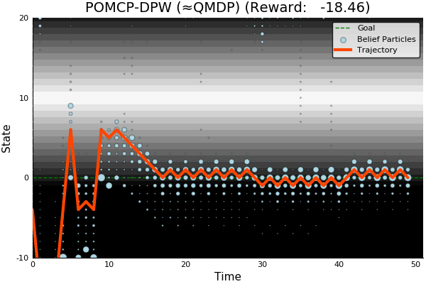
POMCP-DPW


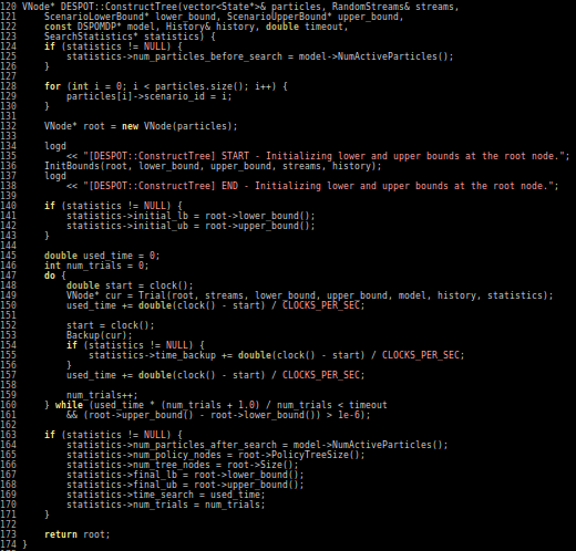
[Sunberg, 2018]
POMDP Solution
QMDP


\[\underset{\pi: \mathcal{B} \to \mathcal{A}}{\mathop{\text{maximize}}} \, V^\pi(b)\]
\[\underset{a \in \mathcal{A}}{\mathop{\text{maximize}}} \, \underset{s \sim{} b}{E}\Big[Q_{MDP}(s, a)\Big]\]
Same as full observability on the next step
POMCP-DPW converges to QMDP
Proof Outline:
-
Observation space is continuous with finite density → w.p. 1, no two trajectories have matching observations
-
(1) → One state particle in each belief, so each belief is merely an alias for that state
-
(2) → POMCP-DPW = MCTS-DPW applied to fully observable MDP + root belief state
-
Solving this MDP is equivalent to finding the QMDP solution → POMCP-DPW converges to QMDP


[Sunberg, 2018]

POMCP-DPW

[ ] An infinite number of child nodes must be visited
[ ] Each node must be visited an infinite number of times
[ ] An infinite number of particles must be added to each belief node
✔
✔
Necessary Conditions for Consistency
Use \(Z\) to insert weighted particles
✔
[Sunberg, 2018]

POMCP
POMCP-DPW
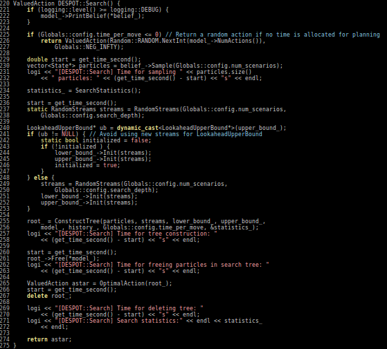
POMCPOW
[Sunberg, 2018]

Ours
Suboptimal
State of the Art
Discretized
[Ye, 2017] [Sunberg, 2018]


[Sunberg, 2018]
Ours
Suboptimal
State of the Art
Discretized


[Sunberg, 2018]
Ours
Suboptimal
State of the Art
Discretized

[Sunberg, 2018]
Ours
Suboptimal
State of the Art
Discretized


[Sunberg, 2018]
Ours
Suboptimal
State of the Art
Discretized

[Sunberg, 2018]

Next Step: Planning on Weighted Scenarios

Driving
POMCPOW
POMDPs.jl
Future
POMDPs
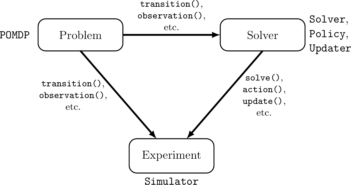
POMDPs.jl - An interface for defining and solving MDPs and POMDPs in Julia
[Egorov, Sunberg, et al., 2017]
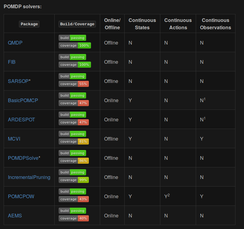
Challenges for POMDP Software
- POMDPs are computationally difficult.
Julia - Speed

Celeste Project
1.54 Petaflops

Challenges for POMDP Software
- POMDPs are computationally difficult.
- There is a huge variety of
- Problems
- Continuous/Discrete
- Fully/Partially Observable
- Generative/Explicit
- Simple/Complex
- Solvers
- Online/Offline
- Alpha Vector/Graph/Tree
- Exact/Approximate
- Domain-specific heuristics
- Problems

Explicit
Black Box
("Generative" in POMDP lit.)
\(s,a\)
\(s', o, r\)
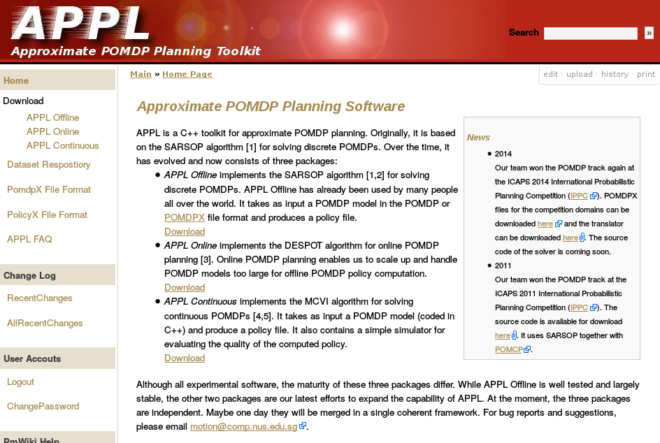
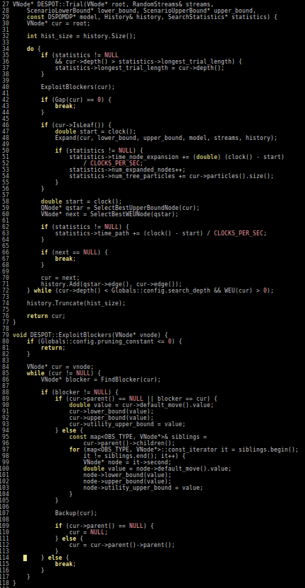
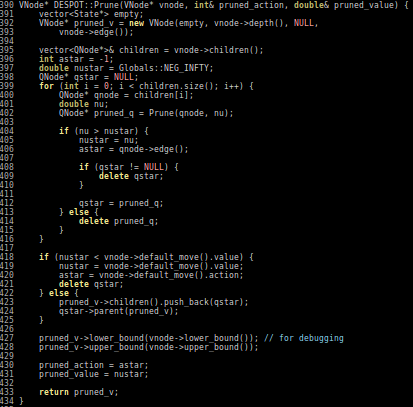
Previous C++ framework: APPL
"At the moment, the three packages are independent. Maybe one day they will be merged in a single coherent framework."
[Egorov, Sunberg, et al., 2017]

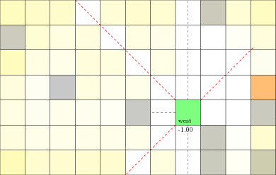
using POMDPs, QuickPOMDPs, POMDPSimulators, QMDP

S = [:left, :right]
A = [:left, :right, :listen]
O = [:left, :right]
γ = 0.95

function T(s, a, sp)
    if a == :listen
        return s == sp
    else # a door is opened
        return 0.5 #reset
    end
end

function Z(a, sp, o)
    if a == :listen
        if o == sp
            return 0.85
        else
            return 0.15
        end
    else
        return 0.5
    end
end

function R(s, a)
    if a == :listen
        return -1.0
    elseif s == a # the tiger was found
        return -100.0
    else # the tiger was escaped
        return 10.0
    end
end

m = DiscreteExplicitPOMDP(S,A,O,T,Z,R,γ)
from julia.QuickPOMDPs import *
from julia.POMDPs import solve, pdf
from julia.QMDP import QMDPSolver
from julia.POMDPSimulators import stepthrough
from julia.POMDPPolicies import alphavectors
S = ['left', 'right']
A = ['left', 'right', 'listen']
O = ['left', 'right']
γ = 0.95
def T(s, a, sp):
if a == 'listen':
return s == sp
else: # a door is opened
return 0.5 #reset
def Z(a, sp, o):
if a == 'listen':
if o == sp:
return 0.85
else:
return 0.15
else:
return 0.5
def R(s, a):
if a == 'listen':
return -1.0
elif s == a: # the tiger was found
return -100.0
else: # the tiger was escaped
return 10.0
m = DiscreteExplicitPOMDP(S,A,O,T,Z,R,γ)Title Text


Driving
POMCPOW
POMDPs.jl
Future
POMDPs
Emerging Research at Stanford and Berkeley
- Trusting Learning-enabled Components
- Active Learning for Safety
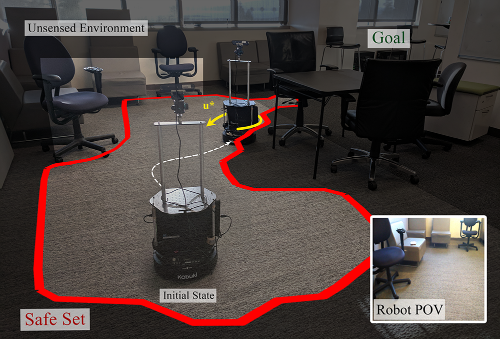
- Safe Planning in Unknown Environments
Trusting Learning-Enabled Components

Environment

Belief State
Convolutional Neural Network
Control System
Architecture for Safety Assurance
Trusting Learning-Enabled Components
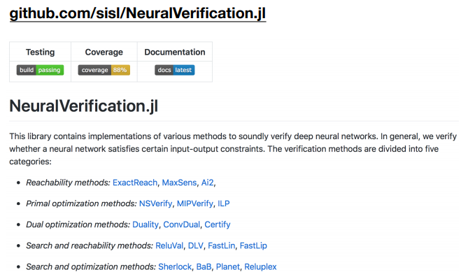
Neural Network Verification
Trusting Learning-Enabled Components
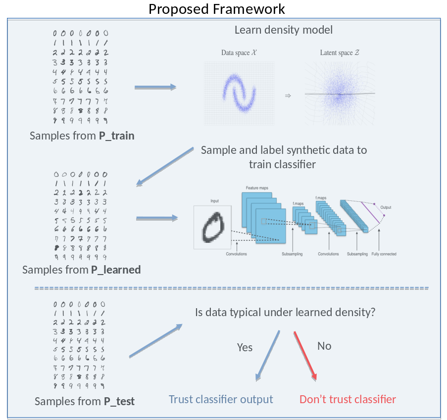
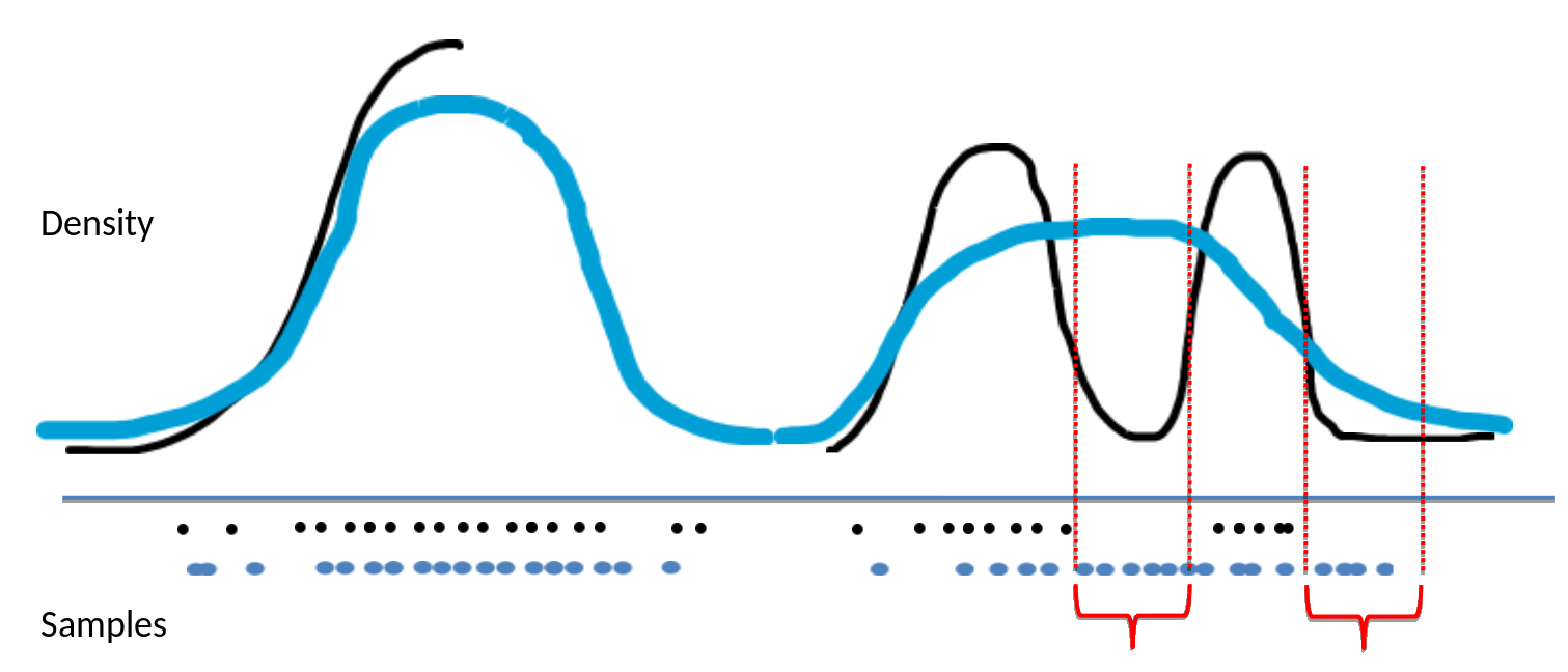
Statistical Trustworthiness of Neural Networks
Active Learning for Safety

?
POMDP
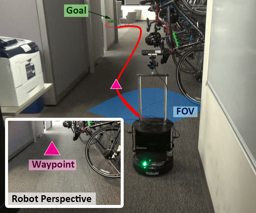
Safe Planning in Unknown Environments
Acknowledgements
The content of my research reflects my opinions and conclusions, and is not necessarily endorsed by my funding organizations.


Thank You!


SRI Talk
By Zachary Sunberg


