Duality in
Structured and Federated Optimization
Zhenan Fan
Department of Computer Science
Supervisor: Michael P. Friedlander
September 14th, 2022
Outline
1
Duality
in
Optimization
Structured
Optimization
Federated
Learning
2
3
Duality in Optimization
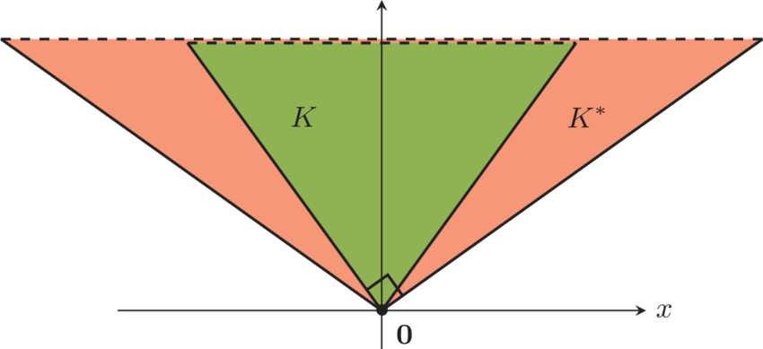

Primal and Dual
Optimization is everywhere
-
machine learning
-
signal processing
-
data mining
Primal problem
Dual problem
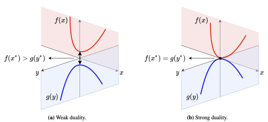
Weak duality
(always hold)
Strong duality
(Under some domain qualification)

Dual Optimization
Possible advantages
-
parallelizable [Boyd et al.'11] -
better convergence rate [Shalev-Shwartz & Zhang.'13] -
smaller dimension [Friedlander & Macêdo'16]
Possible dual formulations
-
Fenchel-Rockafellar dual [Rockafellar'70] -
Lagrangian dual [Boyd & Vandenberghe'04] -
Gauge dual [Friedlander, Macêdo & Pong'04]
(All these different dual formulations can be intepreted using the perturbation framework proposed by [Rockafellar & Wets'98])
Structured Optimization


Structured Data-Fitting
Atomic decomposition: mathematical modelling for structure
[Chen, Donoho & Sauders'01; Chandrasekaran et al.'12]
linear map
observation
sparse low-rank smooth
variables
cardinality
weight
atom
atomic set
- sparse n-vectors
-
low-rank matrices

Example: Separating Stars and Galaxy

[Chen, Donoho & Sauders'98; Donoho & Huo'01]

Example: Separating Chessboard and Chess

[Chandrasekaran et al.'09; Candès et al.'09]

Example: Multiscale Low-rank Decomposition

[Ong & Lustig'16]

Roadmap
Convex relaxation with guarantee
Primal-dual relationship and dual-based algorithm
Efficient primal-retrieval strategy
Fan, Z., Jeong, H., Joshi, B., & Friedlander, M. P. Polar Deconvolution of Mixed Signals. IEEE Transactions on Signal Processing (2021).
Fan, Z., Jeong, H., Sun, Y., & Friedlander, M. P. Atomic decomposition via polar alignment: The geometry of structured optimization. Foundations and Trends® in Optimization (2020).
Fan, Z., Fang, H. & Friedlander, M. P. Cardinality-constrained structured data-fitting problems. Submitted (2022).

Convex Relaxation
Gauge function: sparsity-inducing regularizer [Chandrasekaran et al.'12]
Examples
- sparse n-vectors
-
low-rank matrices
Structured convex optimization [FJJF, IEEE-TSP'21]
Minimizing gauge function can promote atomic sparsity!
structure assumption
data-fitting constraint

Recovery Guarantee
Theorem [FJJF, IEEE-TSP'21]
If the ground-truth signals are incoherent and the measurement are gaussian, then with high probability


Primal-dual Correspondence
Primal problem
Dual problem
Theorem [FSJF, FNT-OPT'21]
Let
and
denote optimal primal and dual solutions. Under mild assumptions,

Dual-based Algorithm
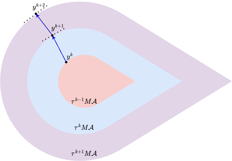
(Projection can be computed approximately using Frank-Wolfe.)
Complexity
projection steps
or
Frank-Wolfe steps
A variant of the level-set method developed by [Aravkin et al.'18]

Primal-retrieval Strategy
Can we retrieve primal variables from near-optimal dual variable?
Theorem [FFF, Submitted'22]
Let
denote the duality gap. Under mild assumptions,
Open-source Package https://github.com/MPF-Optimization-Laboratory/AtomicOpt.jl
(equivalent to unconstrained least square when atomic sets are symmetric)
Federated Learning
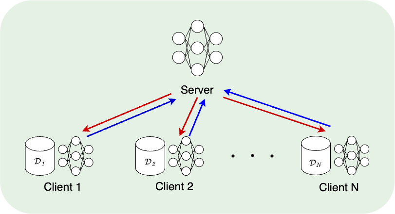

Motivation
Setting
Definition
Federated learning is a collaborative learning framework that can keep data sets private.
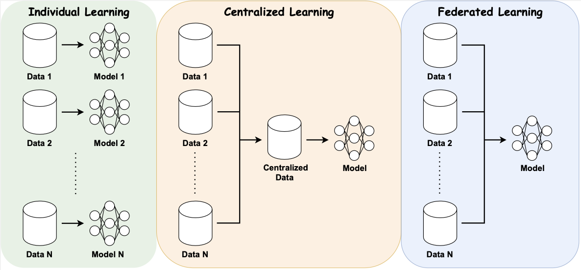
Decentralized data sets, privacy concerns

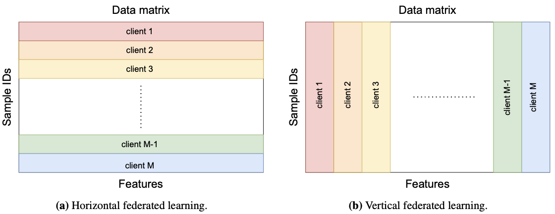
Horizontal and Vertical Federated Learning

Roadmap
Dual-based algorithm for federated optimization
Contribution valuation in federated learning
Fan, Z., Fang, H., Zhou, Z., Pei, J., Friedlander, M. P., Liu, C., & Zhang, Y. Improving Fairness for Data Valuation in Horizontal Federated Learning. IEEE International Conference on Data Engineering (ICDE 2022).
Fan, Z., Fang, H., Zhou, Z., Pei, J., Friedlander, M. P., & Zhang, Y. Fair and efficient contribution valuation for vertical federated learning. Submitted (2022).
Fan, Z., Fang, H. & Friedlander, M. P. FedDCD: A Dual Approach for Federated Learning. Submitted (2022).

Federated Optimization
Important features of federated optimization
-
communication efficiency
-
data privacy
-
data heterogeneity
-
computational constraints
model
number of clients
local dataset
loss function

Primal-based Algorithm
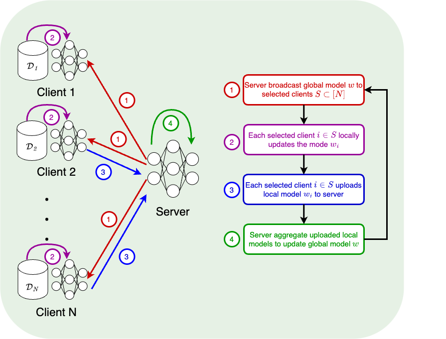
FedAvg [McMahan et al.'17]
SCAFFOLD [Karimireddy et al.'20]

Dual-based Algorithm
Federated dual coordinate descent (FedDCD) [FFF, Submitted'22]
Each selected client approximately compute dual gradient and upload to server
Server adjusts the gradients (to keep feasibility) and broadcasts to selected clients
Each selected client locally updates the dual model
(A extension of [Necoara et al.'17]: inexact gradient, acceleration)
conjugate function
local dual model

Communication Rounds
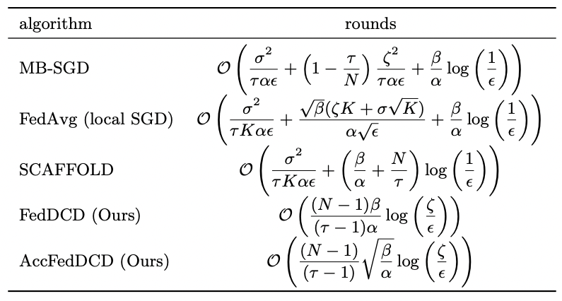
Setting
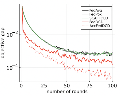
Open-source Package https://github.com/ZhenanFanUBC/FedDCD.jl

Contribution Valuation
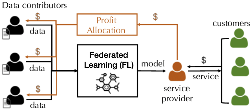
Key requirement
1. Data owners with similar data should receive similar valuation.
2. Data owners with unrelated data should receive low valuation.

Shapley Value
Shapley value is a measure for players' contribution in a game.
Advantage
It satisfies many desired fairness axioms.
Drawback
Computing utilities requires retraining the model.
Previous work
[Wang et al.'20] propose to compute Shapley value in each communication round, which eliminates the requirement of retraining the model.
New drawback
Random selection will cause potential unfairness.
player i
utility created by players in S
marginal utility gain

Our Contribution
[FFZPFLZ, ICDE'22]
We propose a method to improve the fairness. The key idea is to complete a matrix consisting of all the possible contributions by different subsets of the data owners.
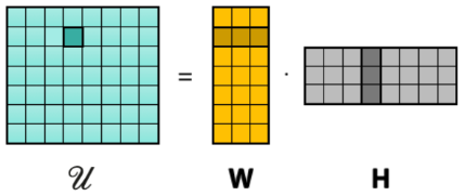
[FFZPFZ, Submitted'22]
We extend this framework to vertical federated learning. (can also be used to determine feature importance)
These two works are partly done during my internship at Huawei Canada. Our code is publicly available at Huawei AI Gallery.

Acknowledgement

Supervisor


University Examiners

External Examiner


Supervisory Committee


Collaborators


