Duality in

Structured and Federated Optimization


Zhenan Fan

Microsoft Research Asia

November 22th, 2022

Outline

1

Duality

in

Optimization

Structured

Optimization

Federated

Learning

2

3

Duality in Optimization
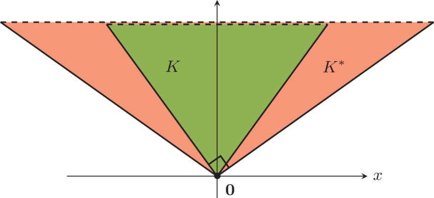
Primal and Dual 

Optimization is everywhere
  • machine learning 
  • signal processing
  • data mining
p^* = \mathop{min}\limits_{x \in \mathcal{X}}\enspace f(x)
Primal problem
Dual problem
d^* = \max\limits_{y \in \mathcal{Y}} \enspace g(y)
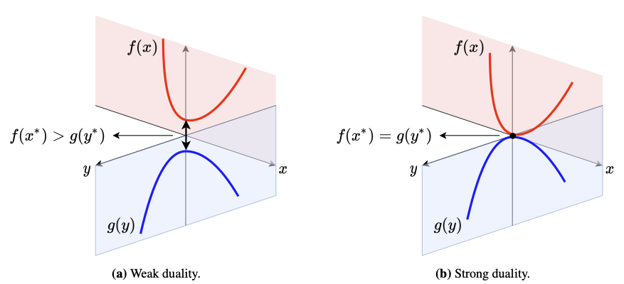
Weak duality
p^* \geq d^*
(always hold)
Strong duality
p^* = d^*
(Under some domain qualification)

Dual Optimization

Possible advantages
  • parallelizable [Boyd et al.'11]
  • better convergence rate [Shalev-Shwartz & Zhang.'13]
  • smaller dimension [Friedlander & Macêdo'16]
Possible dual formulations
  • Fenchel-Rockafellar dual [Rockafellar'70]
  • Lagrangian dual [Boyd & Vandenberghe'04]
  • Gauge dual [Friedlander, Macêdo & Pong'04]
(All these different dual formulations can be intepreted using the perturbation framework proposed by [Rockafellar & Wets'98])

Structured Optimization

Structured Data-Fitting

Atomic decomposition: mathematical modelling for structure

[Chen, Donoho & Sauders'01; Chandrasekaran et al.'12]

\text{Find}\enspace \purple{x_1,\dots,x_k} \in \mathcal{X} \enspace\text{such that}\enspace \red{M}(\sum_{i=1}^k x_i) \approx \blue{b} \enspace\text{and}\enspace x_i \text{ is \green{structured} }\enspace \forall i
linear map
observation
sparse  low-rank  smooth
variables
x = \sum\limits_{j=1}^\purple{\large r} \blue{c_j} a_j, \quad \green{a_j} \in \red{\mathcal{A}}
cardinality
weight
atom
atomic set
  • sparse n-vectors  
  • low-rank matrices
x = \sum_j c_j e_j \quad \mathcal{A} = \{\pm e_1, \dots, \pm e_n\}
X = \sum_j c_ju_jv_j^T \quad \mathcal{A} = \{uv^T \mid \|u\| = \|v\| = 1\}
\green{ x_i \text{ is sparse with respect to } \mathcal{A}_i }

Example: Separating Stars and Galaxy

b
x_1
x_2
\mathcal{A}_1 = \{\pm e_ie_j^T \}
\mathcal{A}_2 = \{ \mathop{DCT}(\pm e_ie_j^T) \}
[Chen, Donoho & Sauders'98; Donoho & Huo'01]

Example: Separating Chessboard and Chess

b
x_1
x_2
\mathcal{A}_1 = \{\pm e_ie_j^T \}
\mathcal{A}_2 = \{uv^T \mid \|u\| = \|v\| = 1\}
[Chandrasekaran et al.'09; Candès et al.'09]

Example: Multiscale Low-rank Decomposition

b
x_1
x_2
x_3
x_4
\mathcal{A}_i = \{uv^T \mid u, v \in \mathbb{R}^{4^{i-1}}, \|u\| = \|v\| = 1\}
[Ong & Lustig'16]

Roadmap

Convex relaxation with guarantee

Primal-dual relationship and dual-based algorithm

Efficient primal-retrieval strategy

Fan, Z., Jeong, H., Joshi, B., & Friedlander, M. P. Polar Deconvolution of Mixed Signals. IEEE Transactions on Signal Processing (2021).
Fan, Z., Jeong, H., Sun, Y., & Friedlander, M. P. Atomic decomposition via polar alignment: The geometry of structured optimization. Foundations and Trends® in Optimization (2020).
Fan, Z., Fang, H. & Friedlander, M. P. Cardinality-constrained structured data-fitting problems. To appear in Open Journal of Mathematical Optimization (2022).

Convex Relaxation

Gauge function: sparsity-inducing regularizer [Chandrasekaran et al.'12]

\gamma_{\mathcal{A}}(x) = \inf\left\{ \sum\limits_{a\in\mathcal{A}}c_a ~\big\vert~ x = \sum\limits_{a\in\mathcal{A}} c_a a, c_a \geq 0 \right\}
Examples
  • sparse n-vectors  
  • low-rank matrices
\mathcal{A} = \{\pm e_1, \dots, \pm e_n\} \quad \gamma_{\mathcal{A}}(x) = \|x\|_1
\mathcal{A} = \{uv^T \mid \|u\| = \|v\| = 1\} \quad \gamma_{\mathcal{A}}(X) = \|X\|_*

Structured convex optimization [FJJF, IEEE-TSP'21]

\{x_i^*\}_{i=1}^k \in \mathop{argmin}\limits_{x_1, \dots, x_k} \left\{ \red{ \max\limits_{i=1,\dots,k} \frac{1}{\lambda_i}\gamma_{\mathcal{A}_i}(x_i) } ~\big\vert~ \blue{ \|M(\sum_{i=1}^k x_i) - b\| \leq \alpha} \right\}
Minimizing gauge function can promote atomic sparsity!
structure assumption
data-fitting constraint

Recovery Guarantee

b = M(\sum_{i=1}^k x_i^\natural) + \eta \in \mathcal{Y}, \quad x_i^\natural \enspace\text{is}\enspace \mathcal{A}_i-\text{sparse}, \quad \|\eta\| \leq \alpha, \quad \lambda_i = \gamma_{\mathcal{A}_1}(x_1^\natural)/\gamma_{\mathcal{A}_i}(x_i^\natural)

Theorem [FJJF, IEEE-TSP'21]

If the ground-truth signals are incoherent and the measurement are gaussian, then with high probability

\|x_i^* - x_i^\natural\| \leq 4\alpha[\sqrt{\mathop{dim}(\mathcal{Y})} - \Delta], \quad \forall i = 1,\dots,k

Primal-dual Correspondence

Primal problem

\mathop{min}\limits_{x_1, \dots, x_k \in \mathcal{X}}\enspace \max\limits_{i=1,\dots,k} \gamma_{\lambda_i\mathcal{A}_i}(x_i) \enspace\text{s.t.}\enspace \|M(\sum_{i=1}^k x_i) - b\| \leq \alpha
\mathcal{O}(k\cdot\mathop{dim}(\mathcal{X})) \enspace\text{storage}

Dual problem

\mathop{min}\limits_{\tau \in \mathbb{R}_+, y \in \mathcal{Y}}\enspace \tau \enspace\text{s.t.}\enspace (y, \tau) \in \mathop{cone}(M\mathcal{A} \times \{1\}) \enspace\text{and}\enspace y \in \mathbb{B}_2(b, \alpha) \enspace\text{with}\enspace \mathcal{A} = \sum_{i=1}^k \lambda_i\mathcal{A}_i
\mathcal{O}(\mathop{dim}(\mathcal{Y})) \enspace\text{storage}

Theorem [FSJF, FNT-OPT'21]

Let 

\{x_i^*\}_{i=1}^k
y^*

and

denote optimal primal and dual solutions. Under mild assumptions, 

\underbrace{ \mathop{supp}(\mathcal{A}_i, x_i^*) }_{\red{ \{a \in \mathcal{A}_i ~\mid~ a \text{ exists in the decomposition of } x_i^*\}}} \subseteq \underbrace{ \mathop{face}(\mathcal{A}_i, z^* \coloneqq M^*(b - y^*))}_{\red{ \{a \in \mathcal{A}_i ~\mid~ \langle a, z^* \rangle \geq \langle \hat a, z^* \rangle \enspace \forall \hat a \in \mathcal{A}_i\}}}

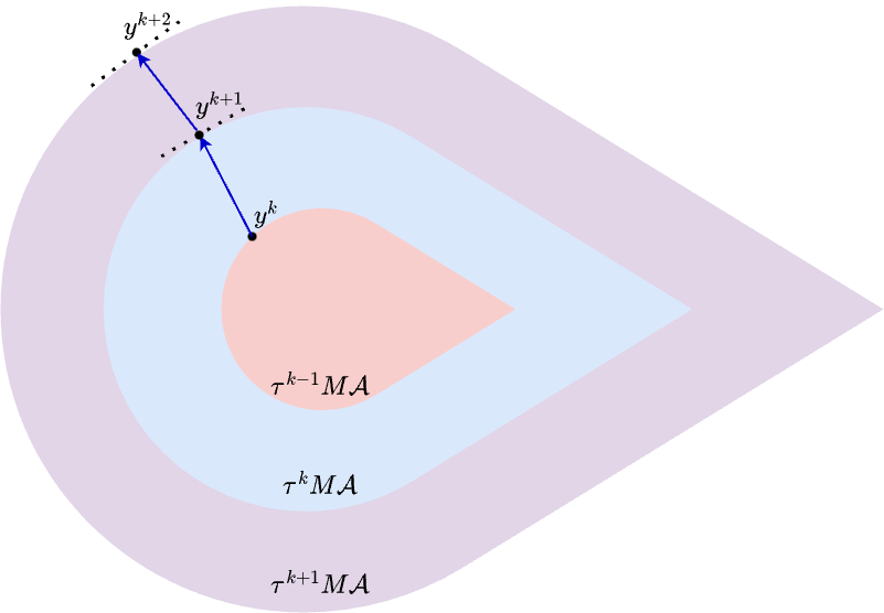
Dual-based Algorithm

y^{k+1} \leftarrow \mathop{Proj}_{\tau^kM\mathcal{A}}(y^k)
\tau^{k+1} \leftarrow \tau^{k} + \frac{\|y^{k+1} - b\| - \alpha}{\sigma_{M\mathcal{A}}(y^{k+1})}
(Projection can be computed approximately using Frank-Wolfe.)

Complexity

\mathcal{O}(\log(1 / \epsilon))
projection steps
or
\mathcal{O}(\log(1 / \epsilon) / \epsilon)
Frank-Wolfe steps
A variant of the level-set method developed by [Aravkin et al.'18]

Primal-retrieval Strategy

Can we retrieve primal variables from near-optimal dual variable?
\{\hat x_i\}_{i=1}^k \in \mathop{argmin}\limits_{x_1, \dots, x_k \in \mathcal{X}} \left\{ \|M(\sum_{i=1}^k x_i) - b\| ~\big\vert~ \mathop{supp}(\mathcal{A}_i; x_i) \in \mathop{face}(\mathcal{A}_i, M^*y) \right\}

Theorem [FFF, Submitted'22]

\epsilon

Let 

denote the duality gap. Under mild assumptions, 

\mathop{cardinality}(\mathcal{A}_i; \hat x_i) \approx \mathop{cardinality}(\mathcal{A}_i; x_i^*) \enspace \forall i \enspace\text{and}\enspace \|M(\sum_{i=1}^k \hat x_i) - b\| \leq \alpha + \mathcal{O}(\sqrt{\epsilon})

Open-source Package https://github.com/MPF-Optimization-Laboratory/AtomicOpt.jl

(equivalent to unconstrained least square when atomic sets are symmetric)

Federated Learning
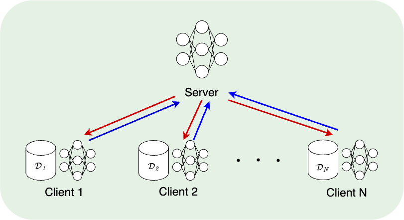
Motivation

Setting
Definition 
Federated learning is a collaborative learning framework that can keep data sets private. 
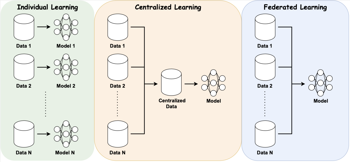
Decentralized data sets, privacy concerns

Horizontal and Vertical Federated Learning
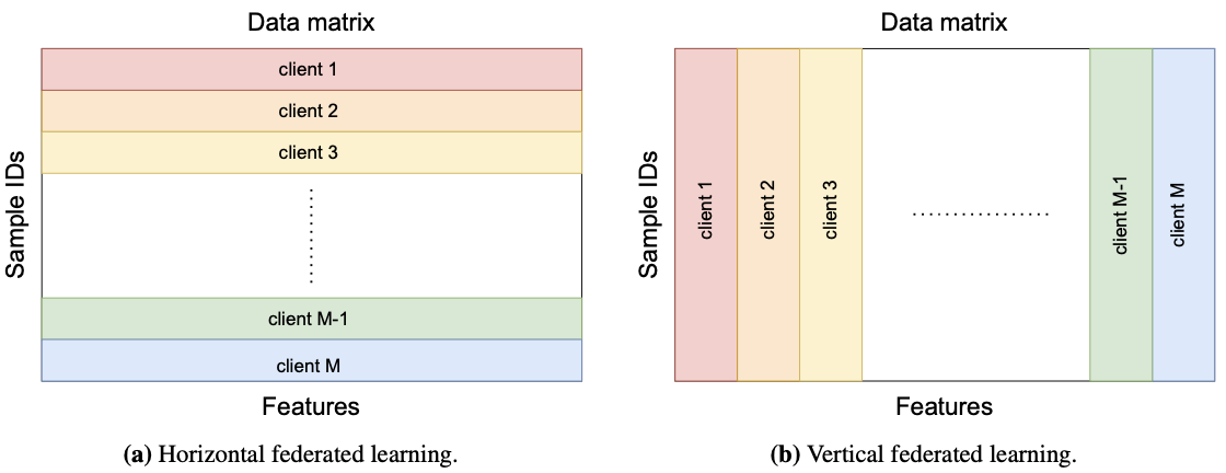
Roadmap

Federated optimization

Fan, Z., Fang, H. & Friedlander, M. P. FedDCD: A Dual Approach for Federated Learning. Submitted (2022).

Knowledge-injected federated learning

Fan, Z., Zhou, Z., Pei, J., Friedlander, M. P., Hu, J., Li, C. & Zhang, Y. Knowledge-Injected Federated Learning. Submitted (2022).

Contribution valuation in federated learning

Fan, Z., Fang, H., Zhou, Z., Pei, J., Friedlander, M. P., Liu, C., & Zhang, Y. Improving Fairness for Data Valuation in Horizontal Federated Learning. IEEE International Conference on Data Engineering (ICDE 2022).
Fan, Z., Fang, H., Zhou, Z., Pei, J., Friedlander, M. P., & Zhang, Y. Fair and efficient contribution valuation for vertical federated learning. Submitted (2022).

Federated Optimization 

Important features of federated optimization
  • communication efficiency
  • data privacy
  • data heterogeneity
  • computational constraints 
\mathop{min}\limits_{w \in \mathbb{R}^d}\enspace F(\red{w}) \coloneqq \sum\limits_{i=1}^\blue{N} f_i(w) \enspace\text{with}\enspace f_i(w) \coloneqq \frac{1}{|\mathcal{D}_i|} \sum\limits_{(x, y) \in \green{\mathcal{D}_i} } \purple{\ell}(w; x, y)
model
number of clients
local dataset
loss function

Primal-based Algorithm
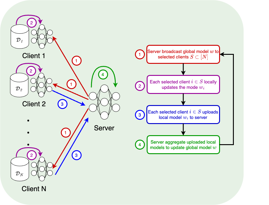
FedAvg [McMahan et al.'17]
w_i \leftarrow w_i - \eta \tilde \nabla f_i(w_i) \quad (K \text{ times})
w \leftarrow \frac{1}{|S|}\sum_{i \in S} w_i
SCAFFOLD [Karimireddy et al.'20]
w_i \leftarrow w_i - \eta (\tilde \nabla f_i(w_i) - c_i + c) \quad (K \text{ times})
c_i \leftarrow \tilde \nabla f_i(w), \enspace c \leftarrow \frac{1}{|S|}\sum_{i \in S} c_i, \enspace w \leftarrow \frac{1}{|S|}\sum_{i \in S} w_i

Dual-based Algorithm

\mathop{min}\limits_{y_1, \dots, y_N \in \mathbb{R}^d}\enspace G(\mathbf{y}) \coloneqq \sum\limits_{i=1}^N \red{f_i^*}(y_i) \enspace\text{subject to}\enspace \sum_{i=1}^N \blue{y_i} = \mathbf{0}
Federated dual coordinate descent (FedDCD) [FFF, Submitted'22]
w_i \approx \nabla f_i^*(y_i) \coloneqq \mathop{argmin}\limits_{w\in \mathbb{R}^d} \{ f_i(w) - \langle w, y_i \rangle \}
\{\hat w_i\}_{i \in S} = \mathop{Proj}_{\mathcal{C}}(\{w_i\}_{i \in S}) \enspace\text{where}\enspace \mathcal{C} = \{ \{v_i \in \mathbb{R}^d\}_{i \in S} \mid \sum_{i \in S} v_i = \mathbf{0}\}
y_i \leftarrow y_i - \eta \hat w_i

Each selected client approximately compute dual gradient and upload to server

Server adjusts the gradients (to keep feasibility) and broadcasts to selected clients

Each selected client locally updates the dual model

(A extension of [Necoara et al.'17]: inexact gradient, acceleration)
conjugate function
local dual model

Communication Rounds
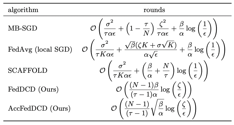
Setting
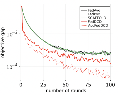
\alpha-\text{strongly convex}, ~\beta-\text{smooth}, ~\zeta-\text{data heterogeneous}, ~\sigma-\text{gradient variance}

Open-source Package https://github.com/ZhenanFanUBC/FedDCD.jl

Knoledge-Injected Federated Learning
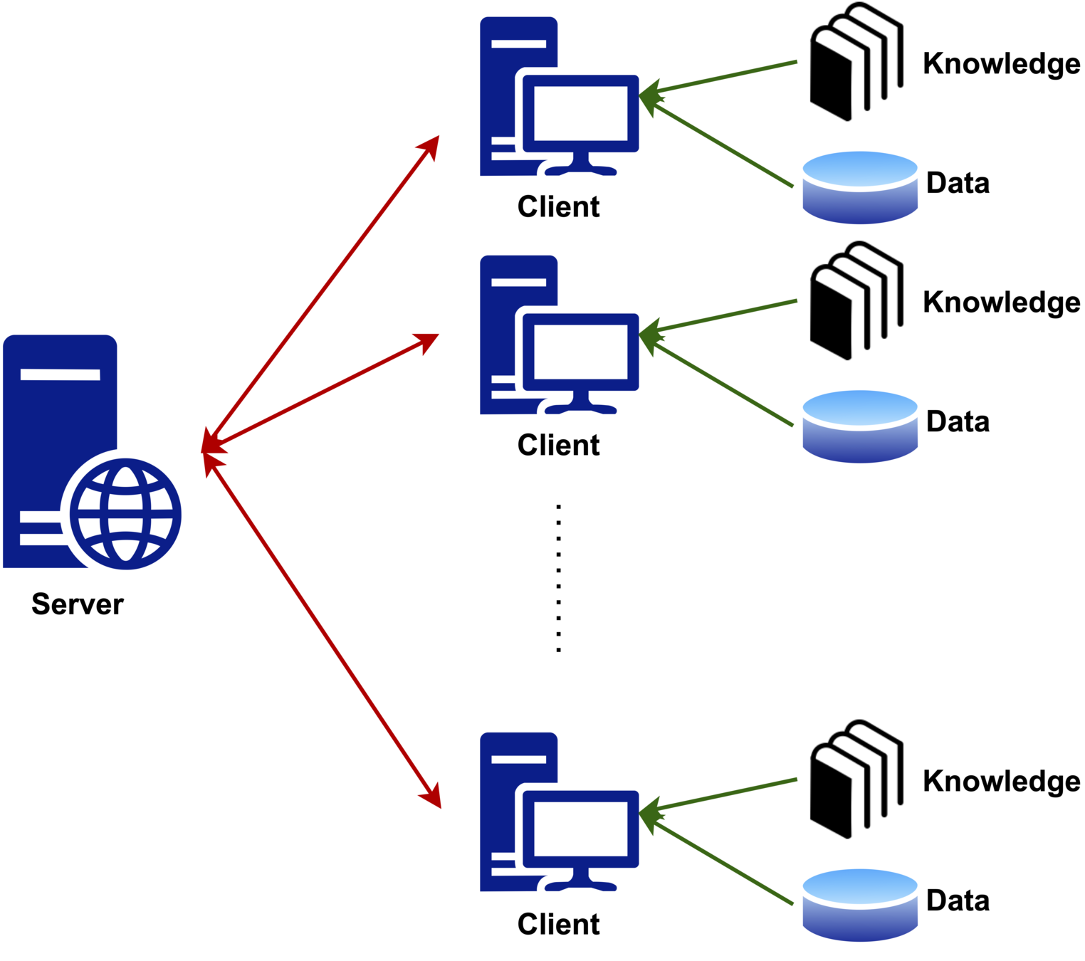
Coal-Mixing in Coking Process
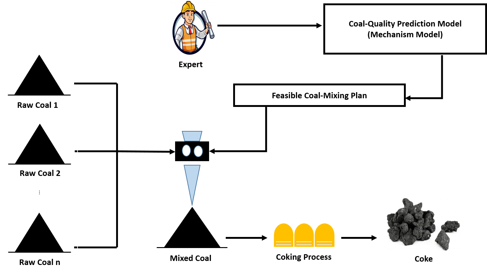
Challenging as no direct formula
Based on experience and knowledge
largely affects cost

Task Description

Goal: improve the expert's prediction model with machine learning
Data scarcity: collecting data is expensive and time consuming
We unite 4 coking industries to collaboratively work on this task
Challeges
local datasets have different distributions
industries have different expert(knowledge) models
privacy of local datasets and knowledge models has to be preserved

Multiclass Classification

\red{\mathcal{D}} = \left\{(\blue{x^{(i)}}, \green{y^{(i)}}\right\}_{i=1}^N \subset \blue{\mathcal{X}} \times \green{\{1,\dots,k\}} \sim \purple{\mathcal{F}}
training set
data instance

(features of raw coal)

feature space
label 
(quality of the final coke)
label space
data distribution
Task
\text{Find}\enspace f: \mathcal{X} \to \{1,\dots,k\} \enspace\text{such that}\enspace \mathop{\mathbb{E}}_{(x,y)\sim\mathcal{F}}[f(x) \neq y] \enspace\text{is small.}
Setting
\enspace\text{or}\enspace \mathop{\mathbb{E}}_{(x,y)\sim\mathcal{D}}[f(x) \neq y] \enspace\text{is small.}

Knowledge-based Models

Prediction-type Knowledge Model (P-KM)
g_p: \mathcal{X} \to \{1,\dots,k\} \enspace\text{such that}\enspace g_p(x) \enspace\text{is a point estimation for}\enspace y \enspace\forall (x,y) \sim \mathcal{F}
Range-type Knowledge Model (R-KM)
g_r: \mathcal{X} \to 2^{\{1,\dots,k\}} \enspace\text{such that}\enspace y \subseteq g_r(x) \enspace\forall (x,y) \sim \mathcal{F}
Eg. Mechanistic prediction models, such as an differential equation that describes the underlying physical process.
Eg. Can be derived from the causality of the input-output relationship.
\red{(k = 3,\enspace g_p(x) = 2)}
\red{(k = 3,\enspace g_r(x) = \{2, 3\})}

Federated Learning with Knowledge-based Models

M clients and a central server.
\text{training set}\enspace \mathcal{D}^m \sim \purple{\mathcal{F}^m}
conditional data distribution depending on
\text{P-KM}\enspace g_p^m \enspace\text{for distribution}\enspace \mathcal{F}^m
\text{R-KM}\enspace g_r^m \enspace\text{for distribution}\enspace \mathcal{F}^m
\purple{\mathcal{F}}
Each client m has
g_p^m \enspace\text{agrees with}\enspace g_r^m \enspace \red{(g_p^m(x) \in g_r^m(x) \enspace \forall x)}

Task Description

each client m obatins a personalized predictive model 
f^m: \mathcal{X} \to \Delta^k \coloneqq \{p \in \mathbb{R}^k \mid \sum p_i = 1\}
f^m \enspace\text{utilize the local P-KM}\enspace g^m_p \enspace\text{with controllable trust level}
f^m \enspace\text{agrees with local R-KM}\enspace g^m_p \enspace\text{i.e.}\enspace \{i \mid f^m(x)_i > 0\} \subseteq g^m_r(x)\enspace \forall x \in \mathcal{X}
Design a federated learning framework such that 
clients can benefit from others' datasets and knowledge 
privacy of local datasets and local KMs needs to be protected

Direct Formulation Invokes Infinitely Many Constraints

Simple setting 
\text{Single client with}\enspace \mathcal{X} = \mathbb{R}^d
\text{Logistic model}\enspace f(\theta; x) = \blue{\mathop{softmax}}(\theta^T x) \enspace\text{with}\enspace \theta\in\mathbb{R}^{d\times k}
\blue{ \mathop{softmax}(z \in \mathbb{R}^k)_i = \dfrac{\exp(z_i)}{\sum_j \exp(z_j)} }
\red{(f(\theta; \cdot): \mathbb{R}^d \to \Delta^k)}
\text{Loss function}\enspace \mathcal{L}(\theta) = \frac{1}{|\mathcal{D}|} \sum\limits_{(x,y) \in \mathcal{D}} \blue{\mathop{crossentropy}}(f(\theta; x), y)
\blue{ \mathop{crossentropy}(p\in\Delta^k, y\in\{1,\dots,k\}) = -\log(p_y) }
Challenging optimization problem
\min\limits_{\theta \in \mathbb{R}^{d\times k}} \enspace \mathcal{L}(\theta) \enspace\text{s.t.}\enspace \{i \mid f(\theta; x)_i > 0\} \subseteq g_r(x) \enspace \forall x \in \mathbb{R}^d
\red{(\text{infinitely many constraints})}

Architecture Design

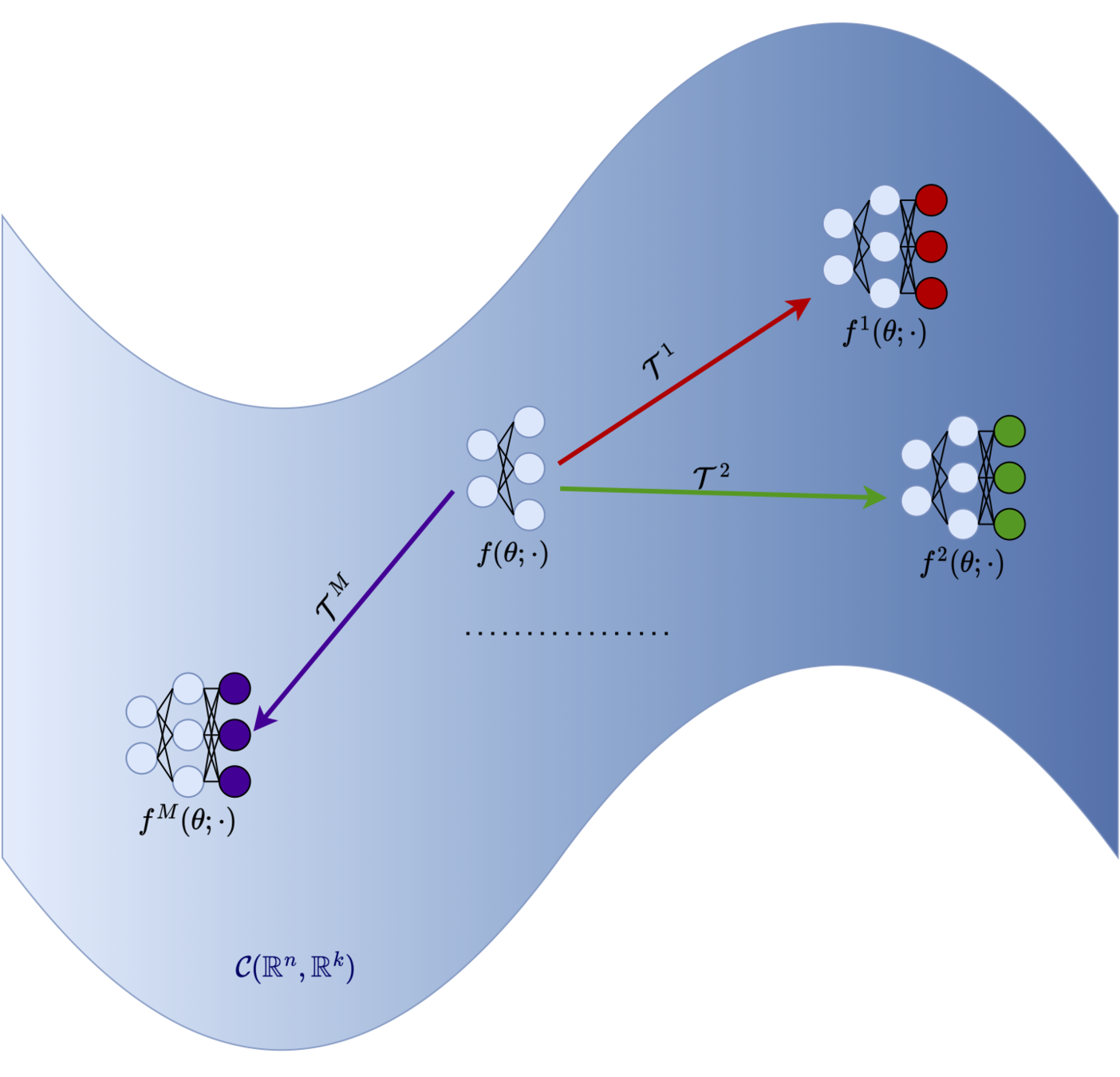
The server provides a general deep learning model
f(\red{\theta}; \cdot): \mathcal{X} \to \mathbb{R}^k
learnable model parameters
Function transformation
\mathcal{T}_{\lambda, g_p, g_r}(f)(x) = (1-\lambda)\mathop{softmax}(f(x) + z_r) + \lambda z_p
where
(z_r)_i = \begin{cases} 0 &\text{if}\enspace i \in g_r(x)\\ -\infty &\text{otherwise} \end{cases} \enspace\text{and}\enspace (z_p)_i = \begin{cases} 1 &\text{if}\enspace i = g_p(x)\\ 0 &\text{otherwise} \end{cases}
Personalized model
f^m(\red{\theta}; \cdot) \coloneqq \mathcal{T}_{\lambda^m, g_p^m, g_r^m}(f(\red{\theta}; \cdot))

Properties of Personalized Model

f^m(\theta; \cdot) \enspace\text{is a valid predictive model, i.e.,}\enspace f^m(\theta; x) \in \Delta^k \enspace \forall x \in \mathcal{X}
\lambda^m \in [0,1] \enspace\text{controls the trust-level of the local P-KM}\enspace g^m_p
\langle f^m(\theta; x), g^m_p(x) \rangle \geq \lambda^m \enspace \forall x \in \mathcal{X}
\text{If}\enspace \lambda^m > 0.5 \enspace\text{then}\enspace f^m \enspace\text{coincides with}\enspace g^m_p
\argmax_i f^m(\theta; x) = g_p^m(x)
f^m(\theta; \cdot) \enspace\text{agrees with local R-KM}\enspace g^m_r
\{i \mid f^m(x)_i > 0\} \subseteq g^m_r(x)\enspace \forall x \in \mathcal{X}

Optimization

Optimization problem 
\min\limits_{\theta}\enspace\red{\mathcal{L}}(\theta) \coloneqq \sum\limits_{i=1}^M \red{\mathcal{L}^m}(\theta) \enspace\text{with}\enspace \mathcal{L}^m(\theta) = \frac{1}{|\mathcal{D}^m|}\sum\limits_{(x,y) \in \mathcal{D}^m} \mathop{crossentropy}(f^m(\theta; x), y)
Eg. FedAvg [McMahan et al.'17]
global loss
local loss
Most existing horizontal federated learning algorithms can be applied to solve this optimization problem!

Numerical Results (Case-study)

Test accuracy 
\text{TA} = \frac{1}{|\mathcal{D}^m_{\text{test}}|} \sum\limits_{(x,y) \in \mathcal{D}^m_{\text{test}}} \mathbb{I}(\{f^m(\theta; x) = y\})
Percentage of violation
\text{POV} = \frac{1}{|\mathcal{D}^m_{\text{test}}|} \sum\limits_{(x,y) \in \mathcal{D}^m_{\text{test}}} \mathbb{I}(\{f^m(\theta; x) \notin g_r^m(x)\})

Open-source Package  https: //github.com/ZhenanFanUBC/FedMech.jl

Contribution Valuation in Federated Learning
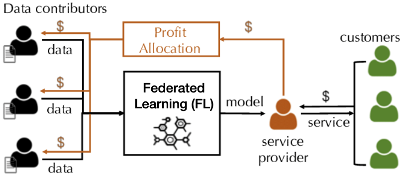
Key requirement 
1. Data owners with similar data should receive similar valuation.
2. Data owners with unrelated data should receive low valuation.

Shapley Value

Shapley value is a measure for players' contribution in a game. 
Advantage 
It satisfies many desired fairness axioms. 
Drawback 
Computing utilities requires retraining the model. 
performance of the model
v(\red{i}) = \frac{1}{N} \sum\limits_{S \subseteq [N] \setminus \{i\}} \frac{1}{ N-1 \choose |S|} [U(S \cup \{i\}) - \blue{U(S)}]
player i
utility created by players in S
marginal utility gain

Horizontal Federated Learning
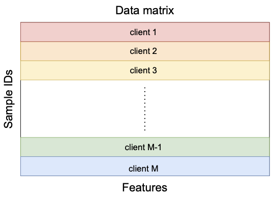
\mathop{min}\limits_{w \in \mathbb{R}^d}\enspace F(\red{w}) \coloneqq \sum\limits_{i=1}^\blue{M} f_i(w) \enspace\text{with}\enspace f_i(w) \coloneqq \frac{1}{|\mathcal{D}_i|} \sum\limits_{(x, y) \in \green{\mathcal{D}_i} } \purple{\ell}(w; x, y)
model
number of clients
local dataset
loss function

Federated Shapley Value

[Wang et al.'20] propose to compute Shapley value in each communication round, which eliminates the requirement of retraining the model. 
v_t(i) = \frac{1}{M} \sum\limits_{S \subseteq [M] \setminus \{i\}} \frac{1}{ M-1 \choose |S|} [U_t(S \cup \{i\}) - U_t(S)]
v(i) = \sum\limits_{t=1}^T v_t(i)
Fairness
Symmetry
U_t(S\cup\{i\}) = U_t(S\cup\{j\}) \quad \forall t, S \Rightarrow v(i) = v(j)
Zero contribution
U_t(S\cup\{i\}) = U_t(S) \quad \forall t, S \Rightarrow v(i) = 0
Addivity
U_t = U^1_t + U^2_t \Rightarrow v(i) = v^1(i) + v^2(i)

Utility Function

Test data set (server)
\mathcal{D}_c
U_t(S) = \sum\limits_{(x, y) \in \mathcal{D}_c} \left[ \ell(w^t; x,y) - \ell(w_S^{t+1}; x,y) \right] \enspace\text{where}\enspace w_S^{t+1} = \frac{1}{|S|} \sum\limits_{i \in S} w_i^{t+1}
v_t(i) = \begin{cases} \frac{1}{|S^t|} \sum\limits_{S \subseteq S^t \setminus\{i\}} \frac{1}{\binom{|S^t|-1}{|S|}} \left[U_t(S\cup\{i\}) - U_t(S)\right] & i \in S^t \\ 0 & i \notin S^t \end{cases}
Problem: In round t, the server only has  
\{w_i^{t+1}\}_{i \in S^t}
[Wang et al.'20] 

Possible Unfairness

Clients with identical local datasets may receive very different valuations.   
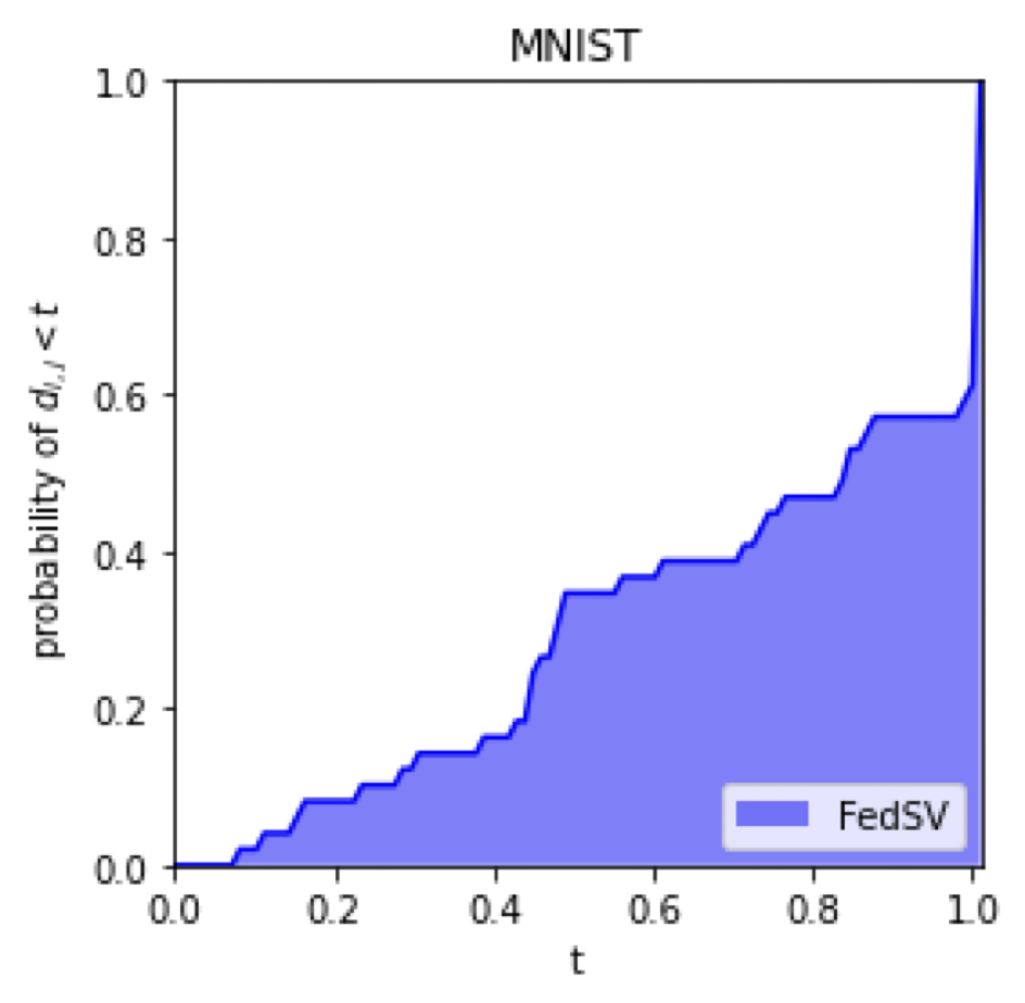
Same local datasets
\mathcal{D}_i = \mathcal{D}_j
Relative difference
d_{i,j} = \frac{|v(i) - v(j)|}{\max\{v(i), v(j)\}}
Empirical probability
\mathbb{P}( d_{i,j} > 0.5) > 65\% \quad \red{\text{unfair!}}

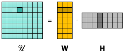
Low Rank Utility Matrix

Utility matrix
\mathcal{U} \in \mathbb{R}^{T \times 2^M} \enspace\text{with}\enspace \mathcal{U}_{t, S} = U_t(S)
This matrix is only partially observed and we can do fair valuation if we can recover the missing values. 

Theorem
If the loss function is smooth and strong convex, then
\red{\mathop{rank}_\epsilon}(\mathcal{U}) \in \mathcal{O}(\frac{\log(T)}{\epsilon})
[Fan et al.'22] 
\red{ \mathop{rank}_\epsilon(X) = \min\{\mathop{rank}(Z) \mid \|Z - X\|_{\max} \leq \epsilon\} }
[Udell & Townsend'19] 

Empirical Results: Singular Value Decomposition

Matrix Completion

\min\limits_{\substack{W \in \mathbb{R}^{T \times r}\\ H \in \mathbb{R}^{2^N \times r}}} \enspace \sum_{t=1}^T\sum_{S\subseteq S^t} (\mathcal{U}_{t,S} - w_t^Th_{S})^2 + \lambda(\|W\|_F^2 + \|H\|_F^2)
Same local datasets
\mathcal{D}_i = \mathcal{D}_j
Relative difference
d_{i,j} = \frac{|v(i) - v(j)|}{\max\{v(i), v(j)\}}
Empirical CDF
\mathbb{P}( d_{i,j} < t)

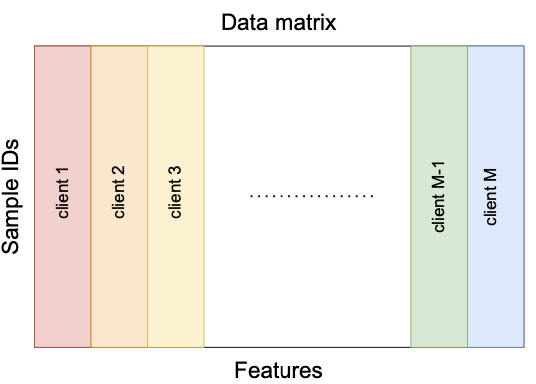
Vertical Federated Learning

\mathop{min}\limits_{\theta_1, \dots, \theta_M}\enspace F(\red{\theta_1, \dots, \theta_M}) \coloneqq \frac{1}{N}\sum\limits_{i=1}^N \ell(\sum_{m=1}^M h^m_i; y_i) \enspace\text{with}\enspace \blue{h^m_i} = \langle \theta_m, x_i^m \rangle
local models
local embeddings
Only embeddings will be communicated between server and clients.   
FedBCD

[Liu et al.'22]
Server selects a mini-batch
B^t \subseteq [N]
Each client m compute local embeddings 
\{ (h_i^m)^t = \langle \theta_m^t, x_i^m \rangle \mid i \in B^t \}
Server computes gradient
\{g_i^t = \frac{\partial \ell(h_i^t; y_i)}{\partial h_i^t} \mid i \in B^t\}
Each client m updates local model 
\theta_m^{t+1} \leftarrow \theta_m^t - \frac{\eta^t}{|B^t|} \sum\limits_{i \in B^t} g_i^t x_i^m

Utility Function

U_t(S) = \frac{1}{N}\sum\limits_{i=1}^N \ell\bigg(\sum\limits_{m=1}^M (h^m_i)^{t-1}; y_i\bigg) - \frac{1}{N}\sum\limits_{i=1}^N \ell\bigg(\sum\limits_{m\in S} (h^m_i)^{t} + \sum\limits_{m\notin S} (h^m_i)^{t-1}; y_i\bigg)
Problem: In round t, the server only has  
\{ (h_i^m)^t \mid i \in B^t \}
Embedding matrix
\mathcal{H}^m \in \mathbb{R}^{T \times N} \enspace\text{with}\enspace \mathcal{H}^m_{t, i} = (h_i^m)^t
Theorem
If the loss function is smooth, then
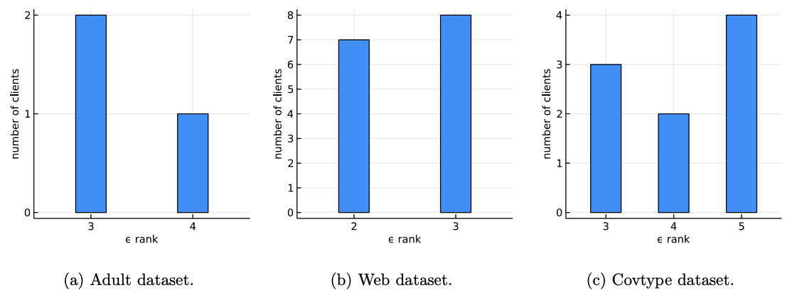
\mathop{rank}_\epsilon(\mathcal{H}^m) \in \mathcal{O}(\frac{\log(T)}{\epsilon})
[Fan et al.'22] 

Empirical Results: Approximate Rank 
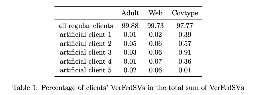
Experiment: Detection of Artificial Clients
These two works are partly done during my internship at Huawei Canada. Our code is publicly available at Huawei AI Gallery.    

Thank you! Questions?

Made with Slides.com