What's in a Prior?

Learned Proximal Networks for Inverse Problems

Zhenghan Fang

CIS Retreat, December 8, 2023

Measure

Inversion

y=Ax+v

Inverse Problems

$A$: Linear forward operator
ill-posed

Inverse Problem in Neuroimaging

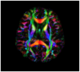
Susceptibility Tensor Images

Dipole Inversion

Dipole Convolution

☹ Time-consuming

Requires >6 orientations

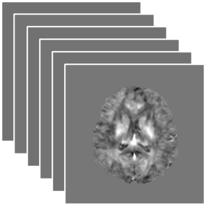
Phase measurements at multiple head orientations

Deep unrolling, Plug-and-play
Use information of physics model
Adaptive to $A$

\min_x \|y - Ax \|_2^2 + R(x)

Regularizer

Classical Method

Not sufficient for few orientations

Learned Proximal

\hat{x}_{k+1} = \mathrm{prox}_{\eta R}(\hat{x}_k - \eta A^H(A\hat{x}_k - y))

Proximal Operator

\hat{x}_{k+1} = {\color{orange} f_\theta}(\hat{x}_k - \eta A^H(A\hat{x}_k - y)) \\

Train $f: X \to Y $ on $\mathcal{D} = (x_i, y_i)_{i=1}^N$

Vanilla Neural Network

Not Adaptable to $A$

$\hat{x} = {\color{orange} f_\theta}(y)$

Learned Proximal for Inverse Problems

$\mathrm{prox}_{\eta R} (z) = \arg\min_u \tfrac{1}{2} \|u-z\|_2^2 + \eta R(u)$

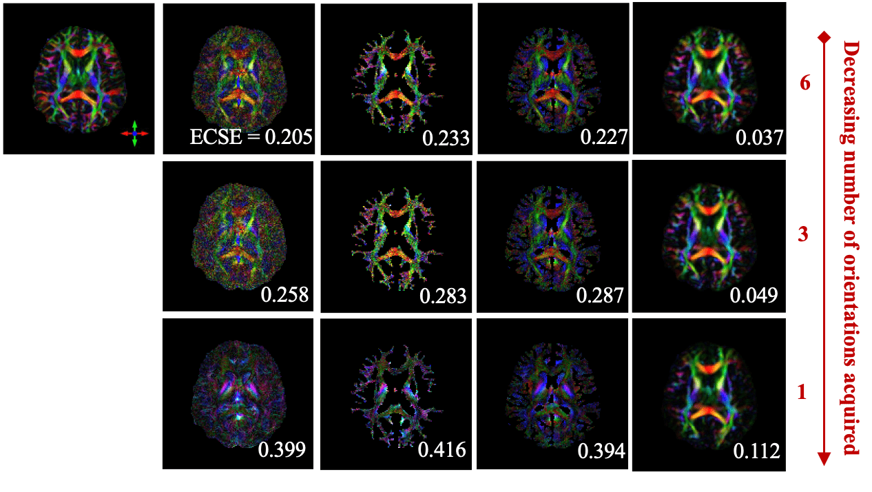
Ground-Truth

STIimag

[Li et al.]

MMSR

[Li and Van Zijl]

aSTI+

[Shi et al.]

DeepSTI

(ours)

[1] Li et al, NMRB 2017; [2] Li and van Zijl, MRM, 2014;

[3] Cao et al., MRM, 2021; [4] Shi et al., IEEE JBHI, 2022

[5] Fang et al. Medical Image Analysis, 2023

Simulation Results

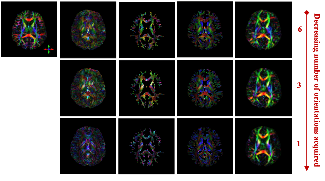
In Vivo Results

DTI

STIimag

[Li et al.]

MMSR

[Li and Van Zijl]

aSTI+

[Shi et al.]

DeepSTI

(ours)

[1] Li et al, NMRB 2017; [2] Li and van Zijl, MRM, 2014;

[3] Cao et al., MRM, 2021; [4] Shi et al., IEEE JBHI, 2022

[5] Fang et al. Medical Image Analysis, 2023

Is $f_\theta$ actually the proximal operator of some function $R_\theta$?
What is the learned regularizer $R_\theta(x)$?

\hat{x}_{k+1} = {\color{orange} f_\theta}(\hat{x}_k - \eta A^H(A\hat{x}_k - y)) \\

Towards Principled and Interpretable Learned Proximal Operator 👉

Characterization of proximal operators [Gribonval and Nikolova, 2020]

Let $f : \mathcal{Y} \rightarrow \R^n$ be a continuous function.

$f$ is a proximal operator of a function $R:\R^n \rightarrow \R \cup \{+\infty\}$

if and only if

there exists a convex differentiable function $\psi$ such that $f(y) = \nabla \psi(y)$.

Proximal operators are gradients of convex functions

Background

Input Convex Neural Networks [Amos et al.]

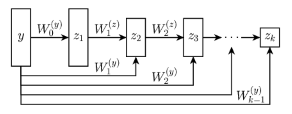
Nonnegative

Learned Proximal Networks

Proposition. Let $\psi_\theta: \R^{n} \rightarrow \R$ be defined by \[z_{1} = g( \mathbf H_1 y + b_1), \quad z_{k} = g(\mathbf W_k z_{k-1} + \mathbf H_k y + b_k), \quad \psi_\theta(y) = \mathbf w^T z_{K} + b\]

with $g$ a convex, non-decreasing nonlinear activation, and all $\mathbf W_k$ and $\mathbf w$ non-negative.

Let $f_\theta = \nabla \psi_{\theta}$.

Then, there exists a function $R_\theta$ such that $f_\theta(y) = \mathrm{prox}_{R_\theta}(y)$.

LPN: Uncovering the Prior

Given $f_\theta$, how can we evaluate $R_\theta$?

$R(x) = \langle x, f^{-1}(x) \rangle - \frac{1}{2} \|x\|_2^2 - \psi(f^{-1}(x))$

\[\min_y \psi_{\theta}(y) - \langle x, y \rangle\]

Optimality condition: $\nabla \psi_\theta(y^*) = x$

[Gribonval and Nikolova]

The minimizer provides the inverse $f_\theta(y^*) = x$

How to invert $f$? 🤔

LPN: Proximal Matching Training

$\mathrm{prox}_{-\log p_x} (y)$

Ideally, $R = -\log p_x$ (MAP estimate)

\min_x \frac{1}{2}\|y - Ax \|_2^2 + R(x)

How to learn? ☹ $p_x$ is unknown

LPN: Proximal Matching Training

$\mathrm{prox}_{-\log p_x} (y)$

Ideally, $R = -\log p_x$ (MAP estimate)

\min_x \frac{1}{2}\|y - Ax \|_2^2 + R(x)

$=\arg\max p(x \mid y)$

$= \arg\min_z \frac{1}{2}\|y - z \|_2^2 -\log p_x (z)$

$x \sim p_x, v \sim \mathcal{N}(0, \mathbf{I}), y = x + \sigma v$

Prox is a MAP denoiser

Learn a MAP denoiser for data

LPN: Proximal Matching Training

$x \sim p_x, v \sim \mathcal{N}(0, \mathbf{I}), y = x + \sigma v$

$\ell2$ $\to$ E[x|y], MMSE

$\ell1 \to$ Median[x|y]

argmax[x|y] ?

$\min_{f} \mathbb{E}_{x,y} \mathcal{L}(f(y), x) $

Train a denoiser $f$:

LPN: Proximal Matching Training

$x \sim p_x, v \sim \mathcal{N}(0, \mathbf{I}), y = x + \sigma v$

$\ell2$ $\to$ E[x|y], MMSE

$\ell1 \to$ Median[x|y]

Theorem (informal). Let
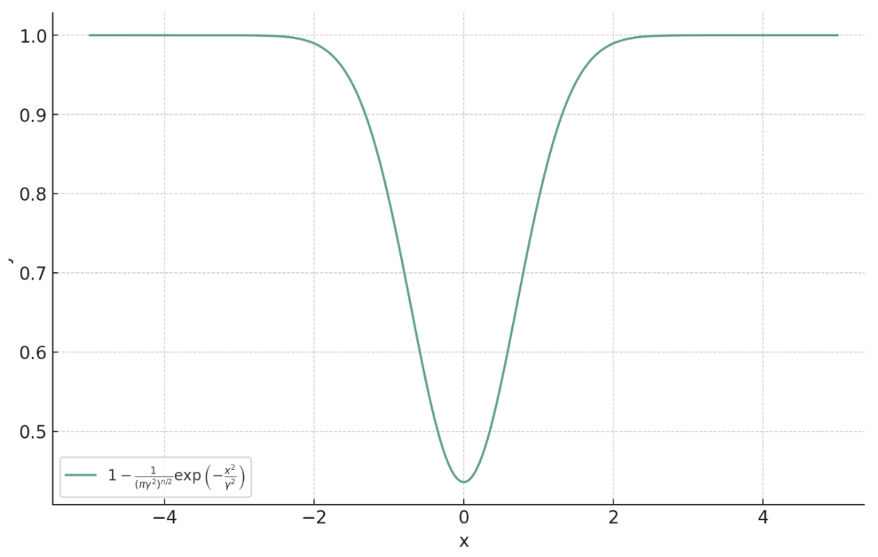
\[f^* = \argmin_{f} \lim_{\gamma \searrow 0} \mathbb{E}_{x,y} \left[ m_\gamma \left( \|f(y) - x\|_2 \right) \right].\]

Then, almost surely (for almost all $y$),

\[f^*(y) = \argmax_{c} p_{x \mid y}(c) = \mathrm{prox}_{-\sigma^2\log p_x}(y).\]

$m_{\gamma}(x) = 1 - \frac{1}{(\pi\gamma^2)^{n/2}}\exp\left(-\frac{x^2}{\gamma^2}\right)$

Prox Matching Loss

Train a denoiser $f$:

$\min_{f} \mathbb{E}_{x,y} \mathcal{L}(f(y), x) $

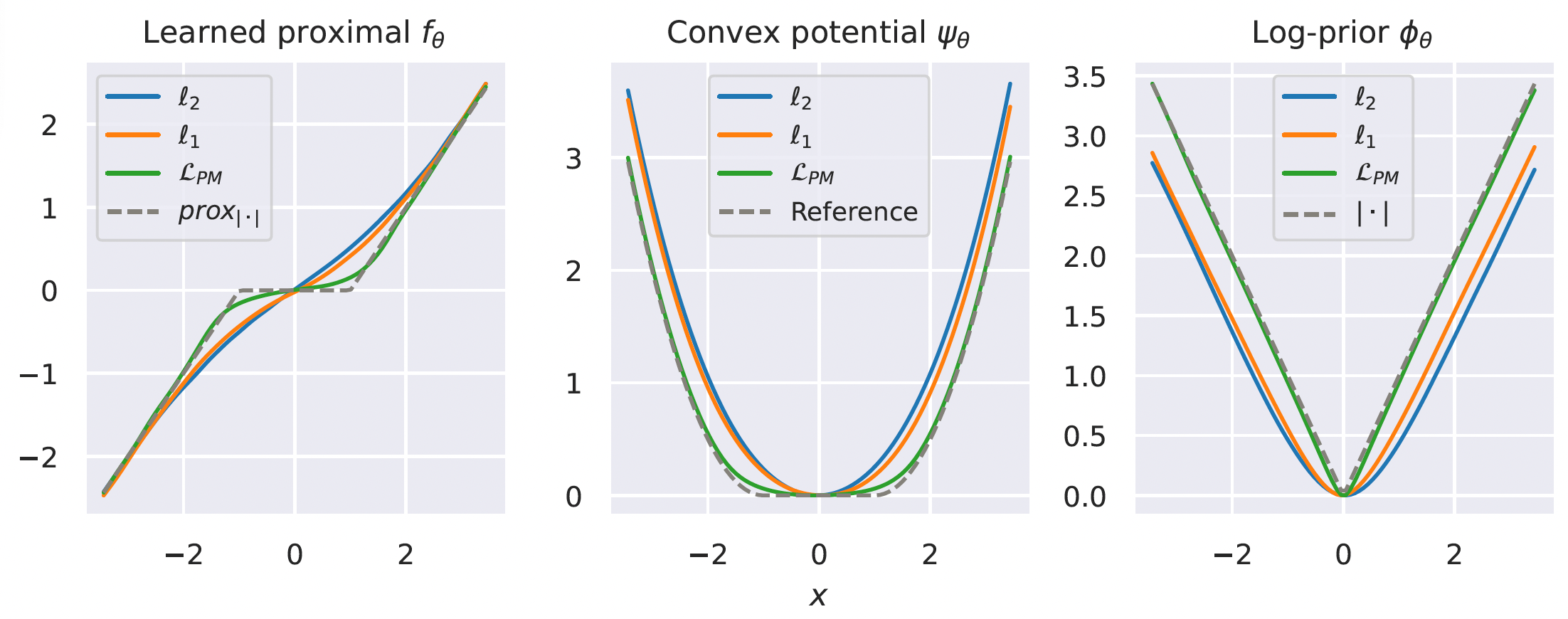
Learning a Prox for the Laplacian

Proximal matching is essential for learning the correct prox/prior

Learning a Prior for Hand-Written Digits

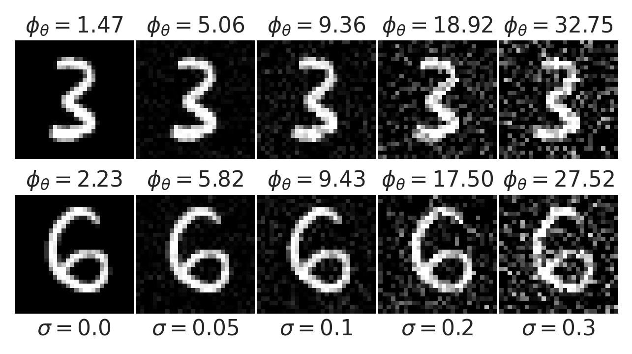
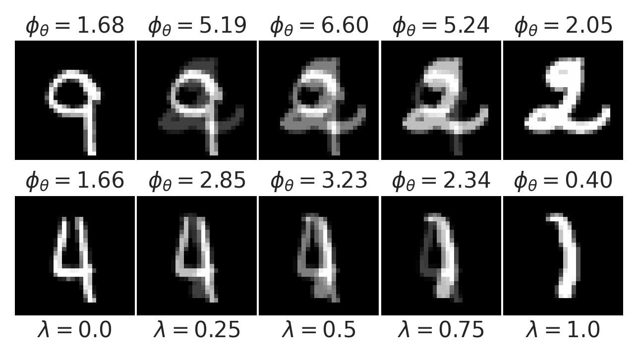
Gaussian noise

Convex interpolation

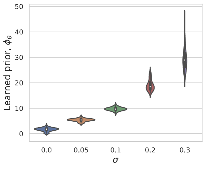
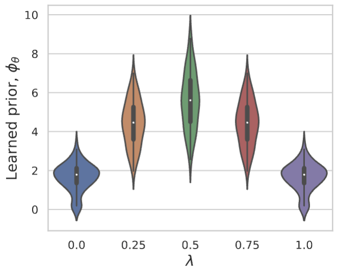
LPN faithfully captures distribution of natural images

Convergence Guarantee with LPN

Then, the iterates $x_k$ converge to a fixed point, $x^*$, that satisfies $f_{\theta}\left(x^* - \eta \nabla h(x^*)\right) = x^*.$ Furthermore, $x^*$ is also a critical point of $h+ \tfrac{1}{\eta} R_\theta$.

Theorem (informal). Let $h(x) = \tfrac{1}{2}\|y - Ax\|_2^2$. Consider the iterates resulting from running LPN with Plug-and-Play and proximal gradient descent:

$$x_{k+1} = f_{\theta}(x_k - \eta \nabla h(x_k)),$$with $0 < \eta < 1/\| A^T A \|$.

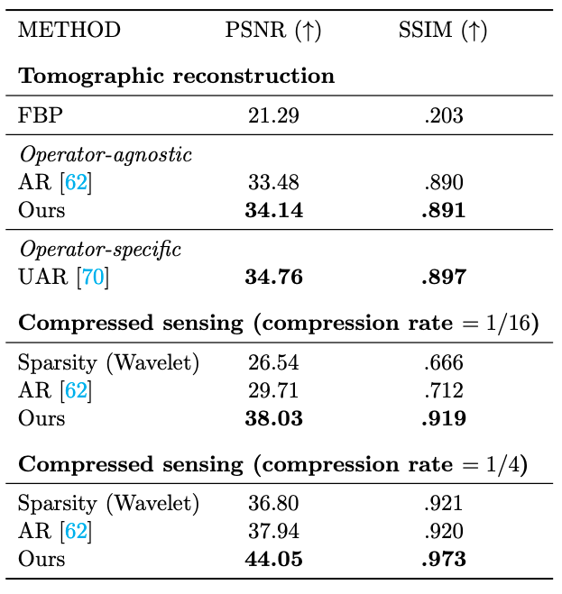
Solving Inverse Problems with LPN

Sparse View Tomographic Reconstruction

Compressed Sensing

Solving Inverse Problems with LPN

Sparse View Tomographic Reconstruction

Compressed Sensing

Summary

A new class of neural networks, learned proximal networks, that guarantee to parameterize proximal operators
- Characterization of implicit priors
A new training paradigm, proximal matching, for learning the proximal of log prior from i.i.d. samples
Convergence guarantees
Competitive performance for inverse problems

Acknowledgements

NIH NIBIB (P41EB031771)
Distinguished Graduate Student Fellows program of the KAVLI Neuroscience Discovery Institute