Identification of Humpback Whales using Deep Metric Learning
Artsiom Sanakoyeu
PhD candidate, Computer Vision Group
Kaggle Master (45-th out of 113.000+)


Content
- Introduction
- Metric Learning Overview
- Sampling For Metric Learning
-
Divide and Conquer the Embedding Space for Metric Learning (CVPR 2019)
- Kaggle Humpback Whale Identification Challenge
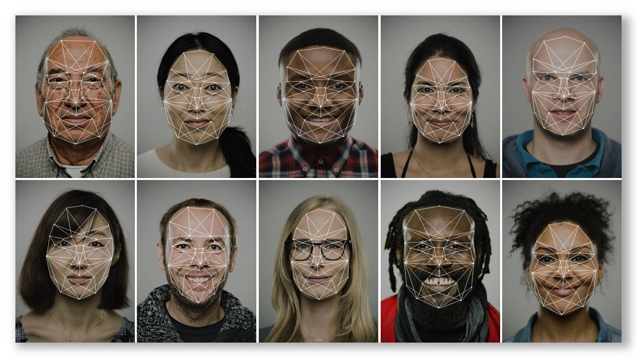
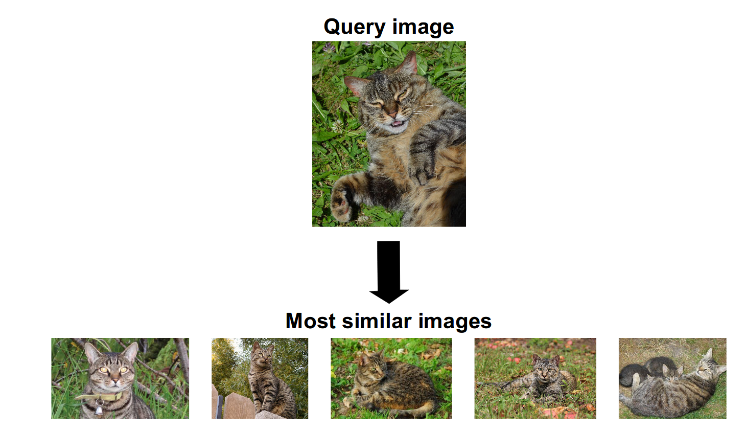
How to compare images?

How similar/dissimilar are these images?
How to compare images?
How to compare images?
Project images in d-dimensional Euclidean space where distances directly correspond to a measure of similarity
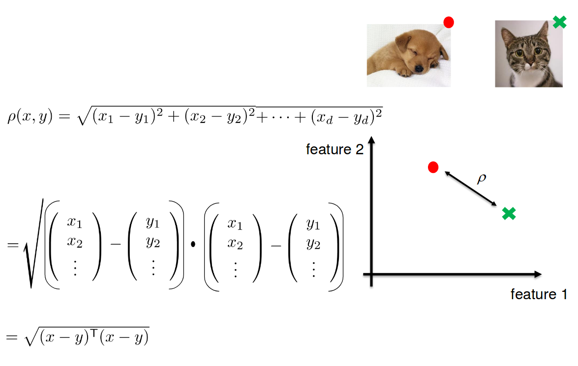

How to compare images?
Metric Learning
Basic idea: learn a metric that assigns small (resp. large) distance to pairs of examples that are semantically similar (resp. dissimilar).


Metric Learning
d-dimensional Embedding Space
How to compare images?
Metric Learning
Basic idea: learn a metric that assigns small (resp. large) distance to pairs of examples that are semantically similar (resp. dissimilar).
Metric Learning
d-dimensional Embedding Space
Small distance
How to compare images?
Metric Learning
Basic idea: learn a metric that assigns small (resp. large) distance to pairs of examples that are semantically similar (resp. dissimilar).
Metric Learning
d-dimensional Embedding Space
Large distance
Metric Learning Applications
Handwriting recognition
Person identification
Image Search
Metric Learning Applications
Deep Metric Learning (DML)
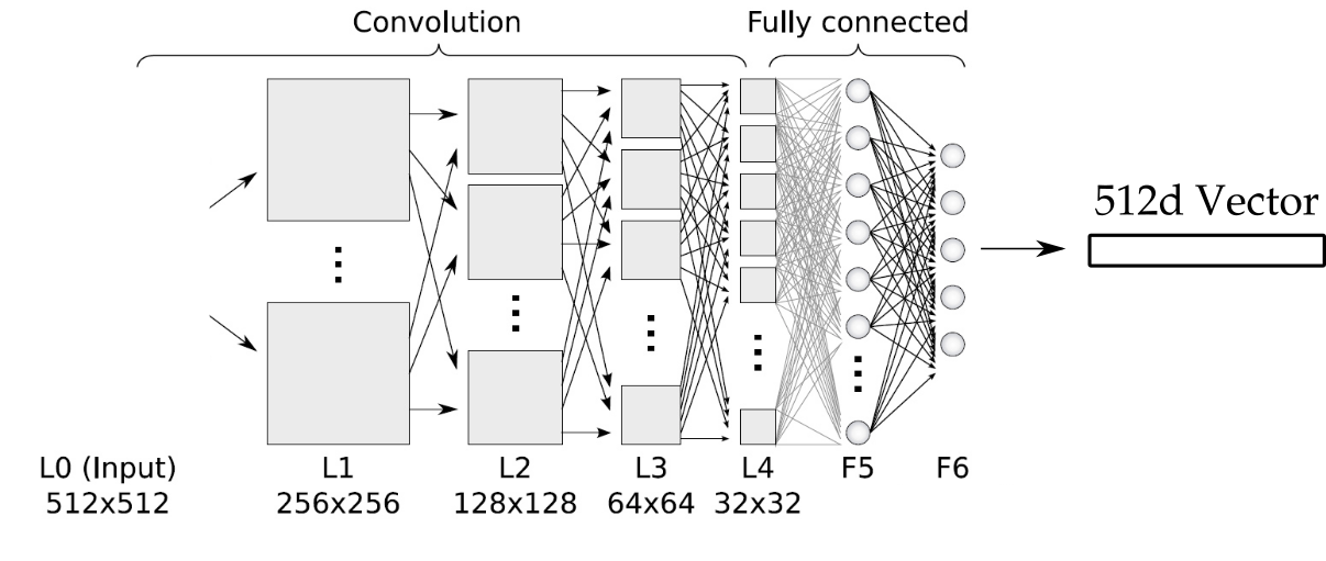
Project Image in d-dimensional space where Euclidean distance would make sense
Deep Metric Learning (DML)
- Each layer to compose the representations of the previous layer to learn a higher level abstraction
- Map from the image space into feature (embedding) space ℝd
Pixels -> Edges -> Contours -> Object parts -> Embedding Space ℝd - Local Features -> Global Features
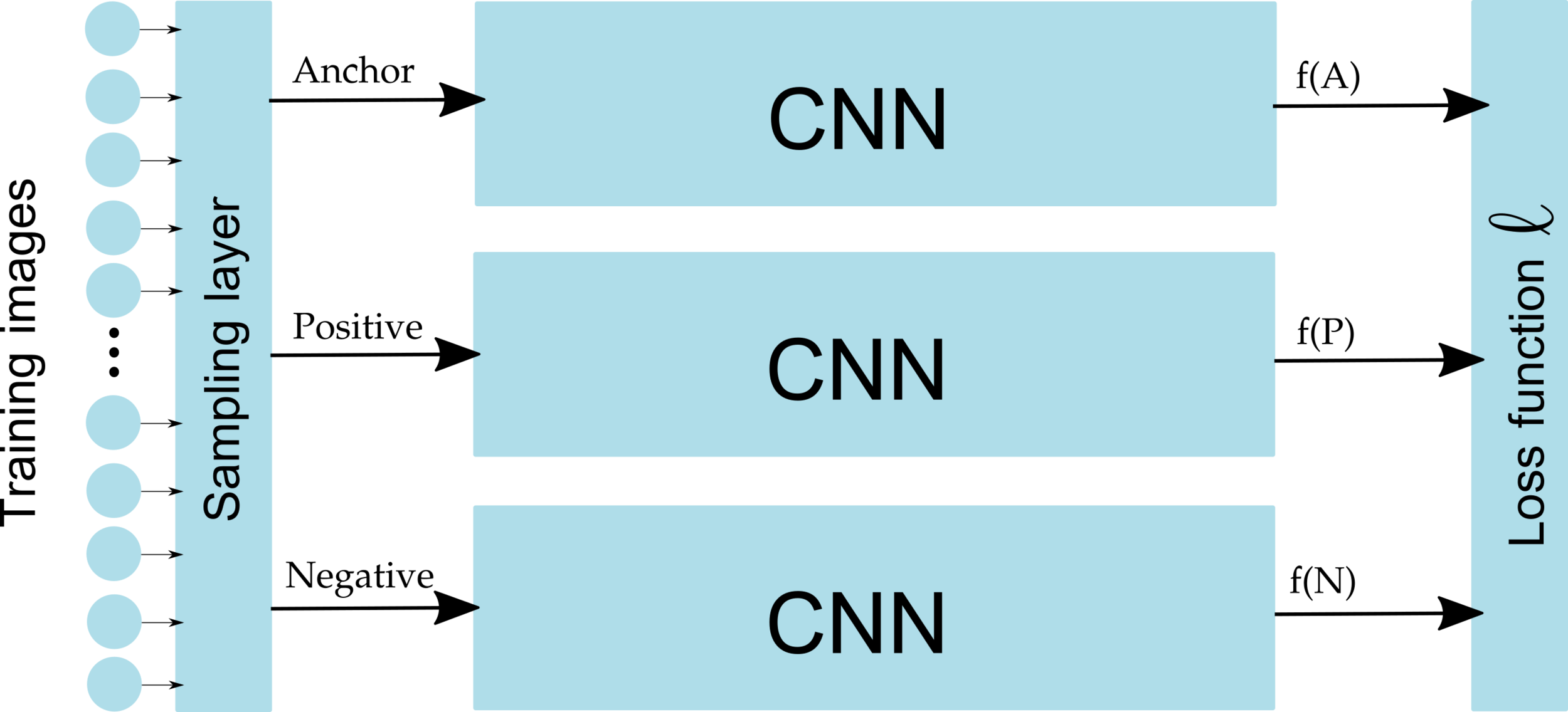
Training: Triplet Loss
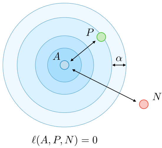
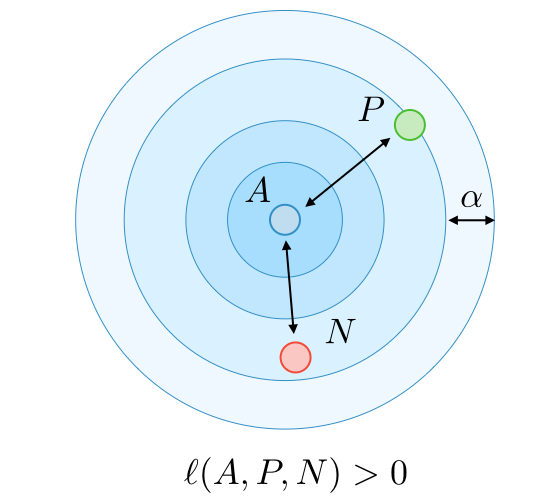
Courtesy: cs-230 course, Stanford University
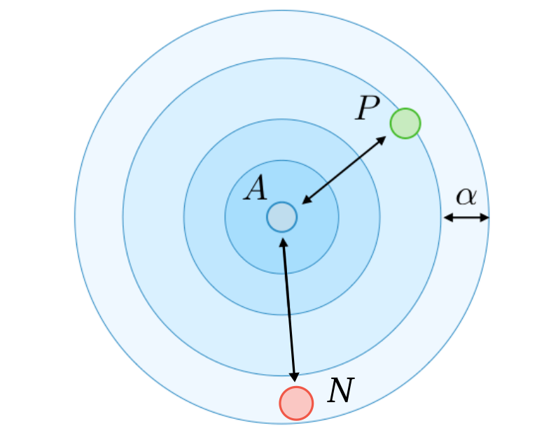
A = Anchor
P = Positive
N = Negative
Training: Siamese Network
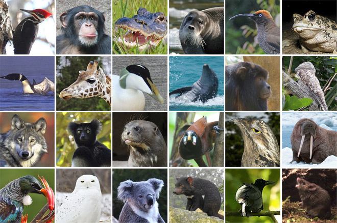
Ex: Learn a Distance Metric for Animals Dataset
Why sampling?
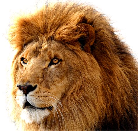
Leopard
Lion
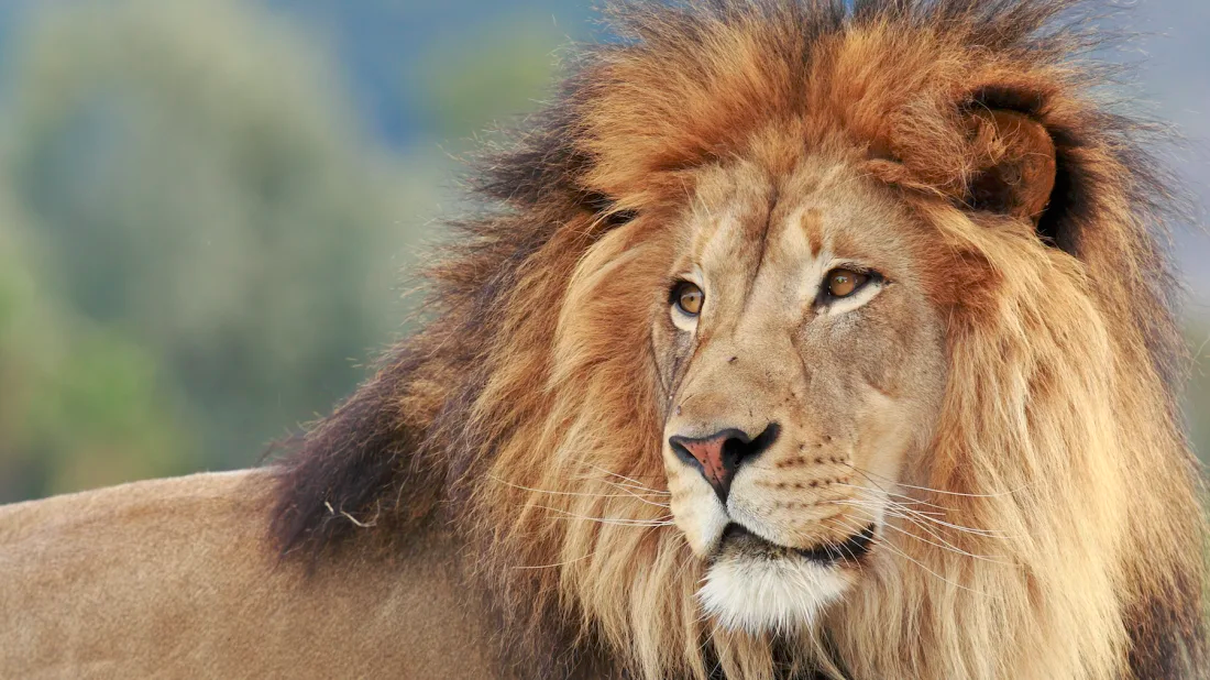
Easy!
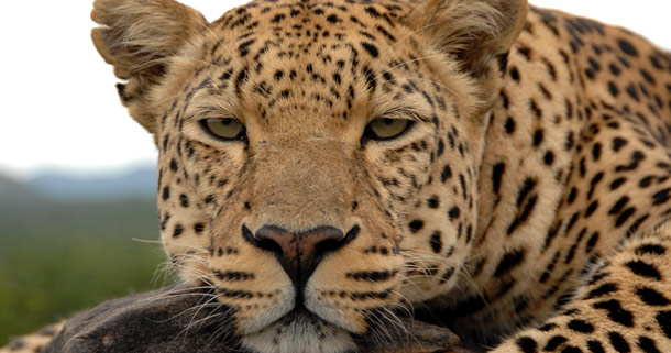
Why sampling?
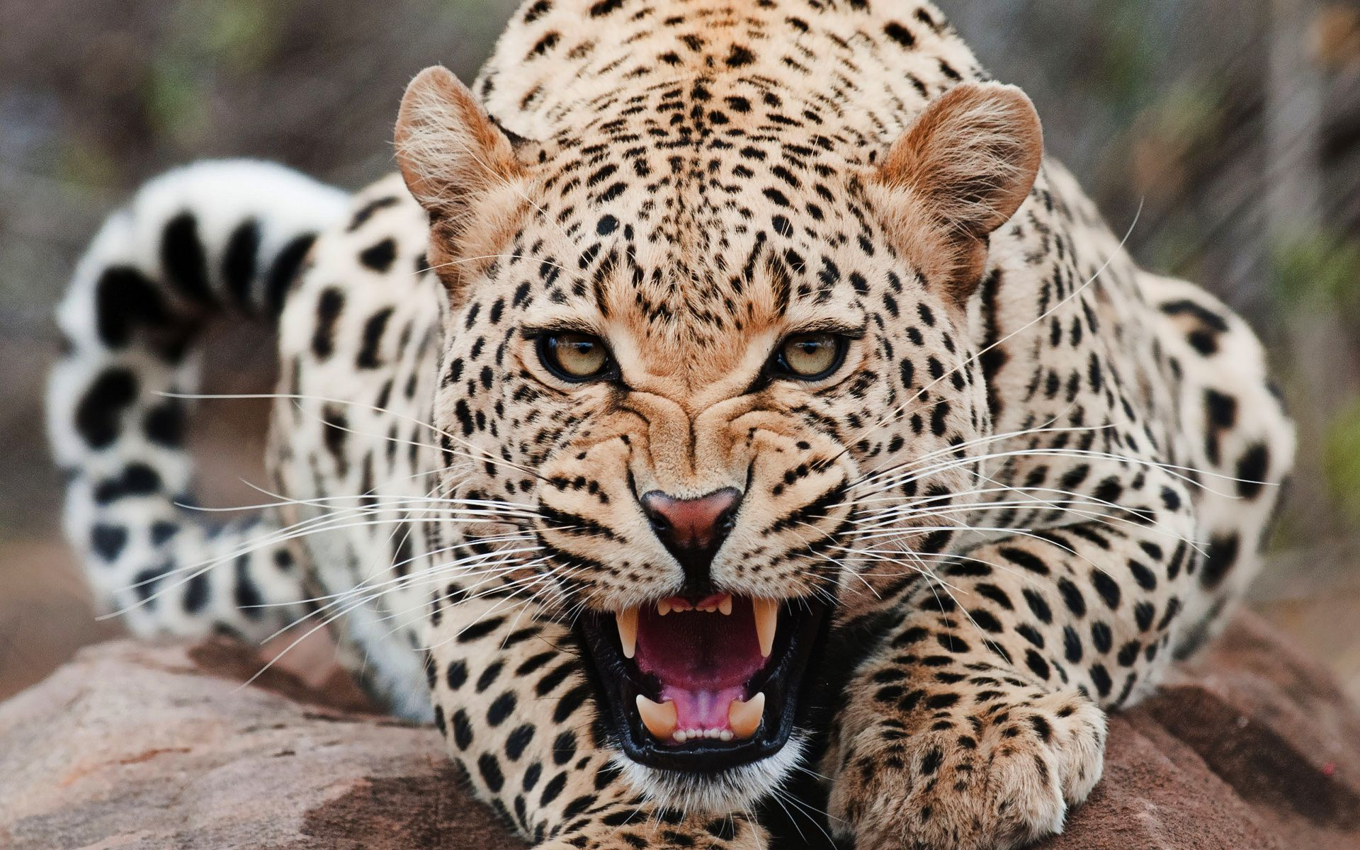
Leopard
Jaguar
Difficult!
Why sampling?
Sampling Layer
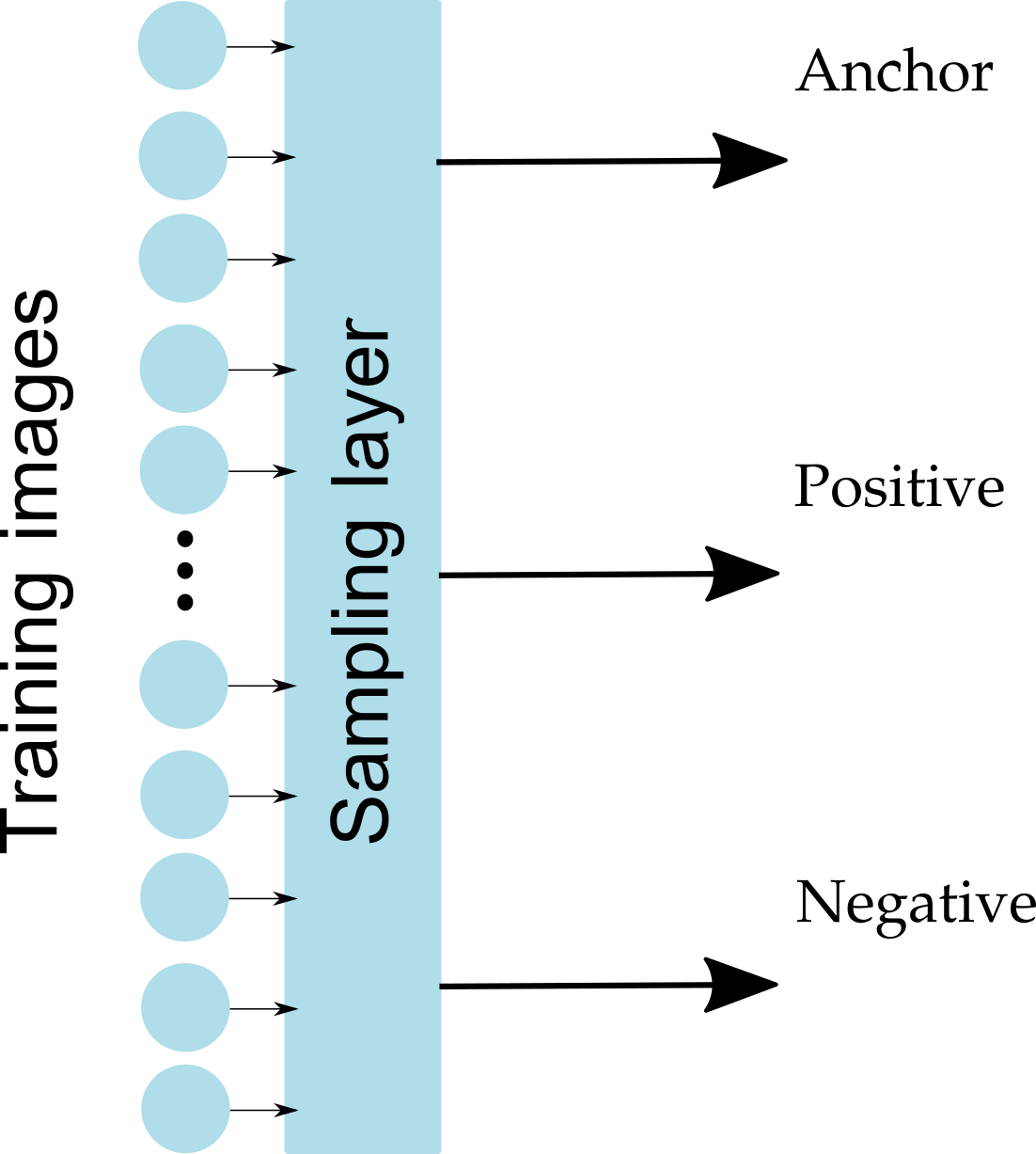
possible triplets in the dataset
Sample randomly?!
NO. Only small portion of all triplets is meaningful and has non-zero loss
Sampling Layer
possible triplets in the dataset
Sample randomly?!
NO. Only small portion of all triplets is meaningful and has non-zero loss
Sample only meaningful triplets!
It’s important to select “hard” triplets (which would contribute to improving the model) to use in training. How do we do that?
Hard Negative Sampling
Sample "hard" (informative) triplets, where loss > 0
Sampling must select different triplets as training progresses
Hard Negative Sampling
-
An idea: Given an anchor image A, select the “hardest” positive image (of the same class) as P (i.e. the one that’s furthest away in the dataset) and select the “hardest” negative image (of a different class) as N (i.e. the one that’s closest in the dataset).
-
Problem: Infeasible to compute these argmax and argmin across the whole dataset. Also this might lead to poor training (considering that mislabeled images and outliers would dominate the hard positives and negatives).
-
Solution: Generate triplets online.
Select P and N (argmax and argmin) from a mini-batch (not from the entire dataset) for each anchor A.
[*] FaceNet: A Unified Embedding for Face Recognition and Clustering, Schroff et al., 2015
Hard Negative Sampling
Hard triplet
1. Gradient with respect to negative example f(N) takes form of
- some function
determines the gradient direction.
Hard Negative Sampling
Hard triplet
1. Gradient with respect to negative example f(N) takes form of
determines the gradient direction. Dominated by noise if is too small
- some function
noise
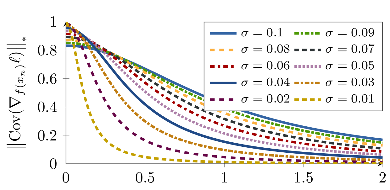
Variance of gradient at different noise levels
Sampling Matters in Deep Embedding Learning, Wu et al., ICCV 2017
Hard Negative Sampling
Hard triplet
2. Selecting the hardest negatives can in practice lead to bad local minima early on in training, specifically it can result in a collapsed model (i.e. f(x) = 0) [1].
[1] FaceNet: A Unified Embedding for Face Recognition and Clustering, Schroff et al., 2015
Semi-hard Negative Sampling
Semi-Hard triplet
Hard triplet
Semi-hard Negative Sampling
Semi-Hard triplet
Semi-hard Negative Sampling is not The Best
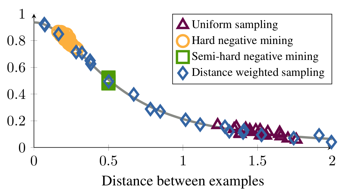
Fig. 2: Distribution of distances between anchor and negative for different strategies
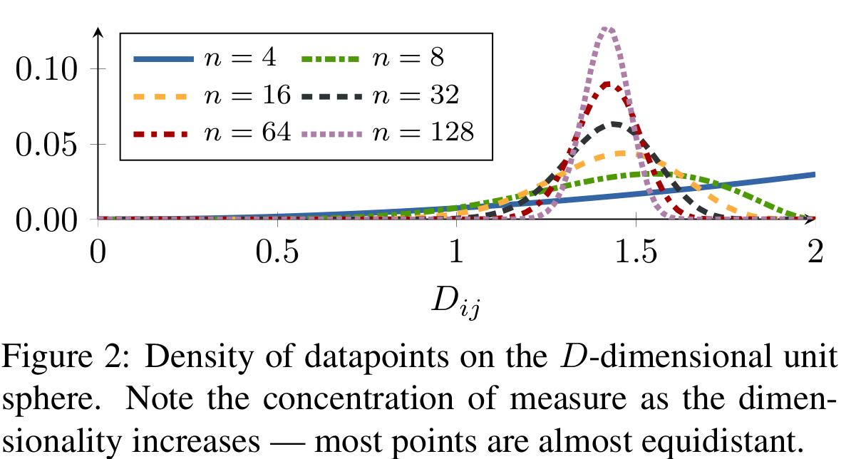
Fig. 1: Density of datapoints on the n-dimensional unit
sphere. Note the concentration of measure as the dimensionality increases — most points are almost equidistant.
Variance of gradient

Distance weighted sampling
Sampling Matters in Deep Embedding Learning, Wu et al., ICCV 2017
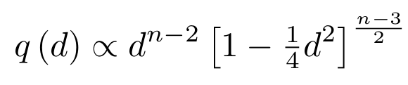
Margin Loss
Sampling Matters in Deep Embedding Learning, Wu et al., ICCV 2017
Triplet Loss
Loss for positive pairs
Loss for negative pairs
Triplet Loss
Margin Loss
Conclusion
To learn image similarities:
- Use Siamese Networks
- Triplet Loss / Margin Loss
- Triplets sampling (offline / online):
- Hard negative mining
- Semi-hard negative mining
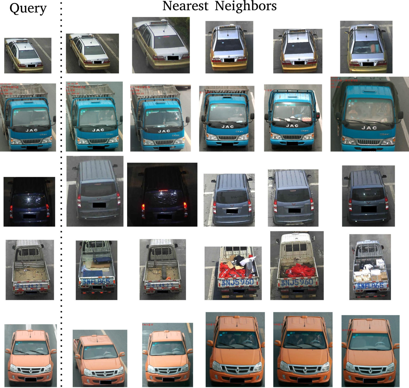
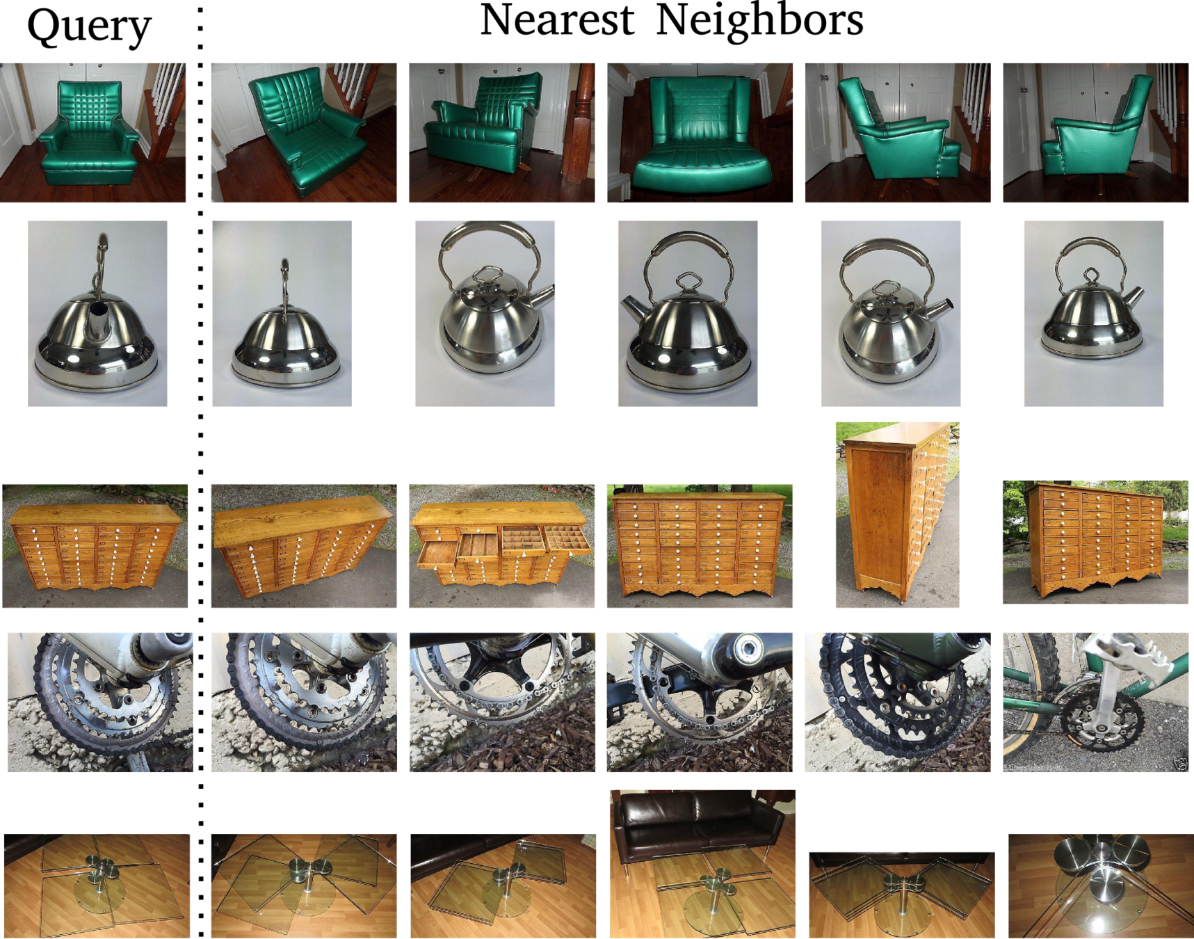
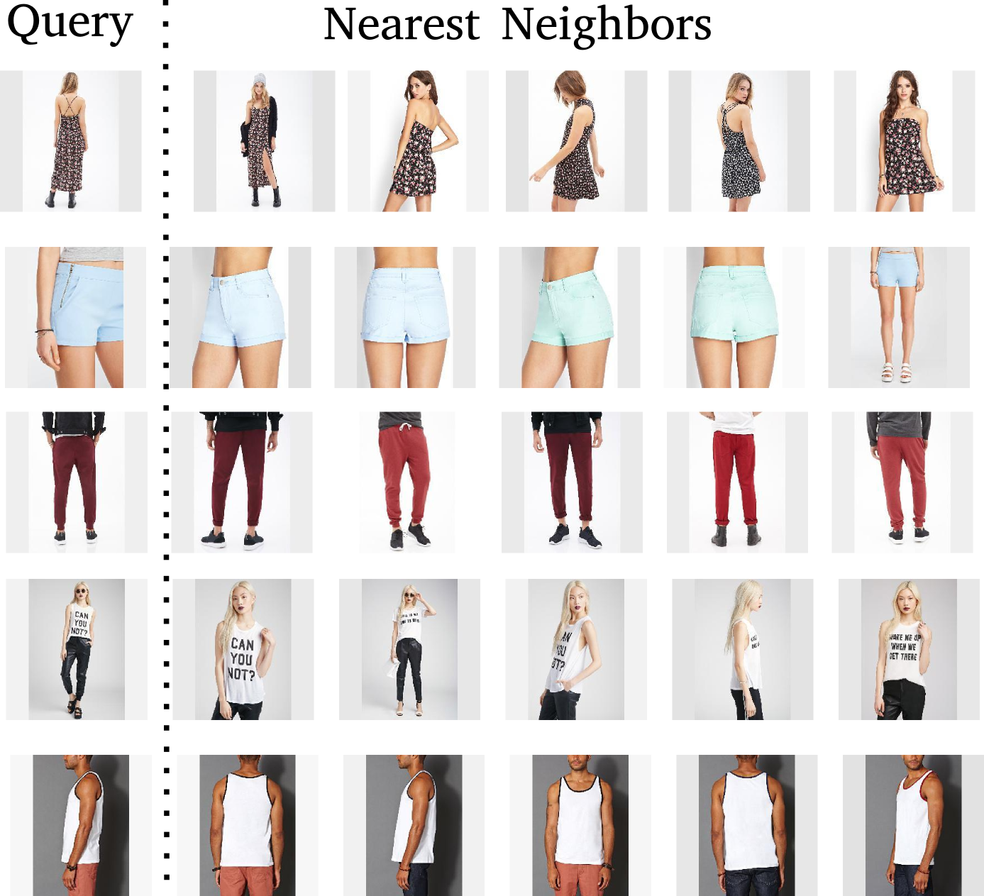
Divide and Conquer the Embedding Space for Metric Learning
Artsiom Sanakoyeu*, Vadim Tschernezki*, Uta Büchler, Björn Ommer
CVPR 2019
Universal approximation theorem:
A feed-forward network with a single hidden layer containing a finite number of neurons can approximate continuous functions on compact subsets of R, under mild assumptions on the activation function — Wikipedia
In simple terms: you can always come up with a deep neural network that will approximate any complex relation between input and output.
Motivation: Representational Power of Deep Neural Networks
IN PRACTICE: It is extremely difficult to get an optimal solution since the objective function is highly non-convex. We always get stuck in local optima.
~
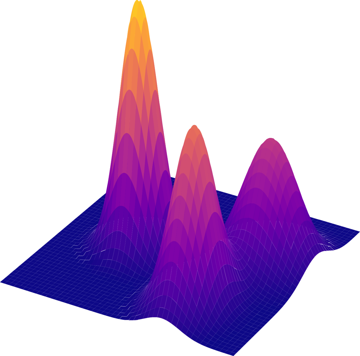
Motivation: Data distribution is complex and multimodal
~
Motivation: Data distribution is complex and multimodal
Existing Approaches: Learn a single distance metric for all training data
→ Overfit and fail to generalize well.
~
Existing Approaches: Learn a single distance metric for all training data
→ Overfit and fail to generalize well.
To alleviate this problem: Learn several different distance metrics on non-overlaping subsets of the data.
Motivation: Data distribution is complex and multimodal
Method
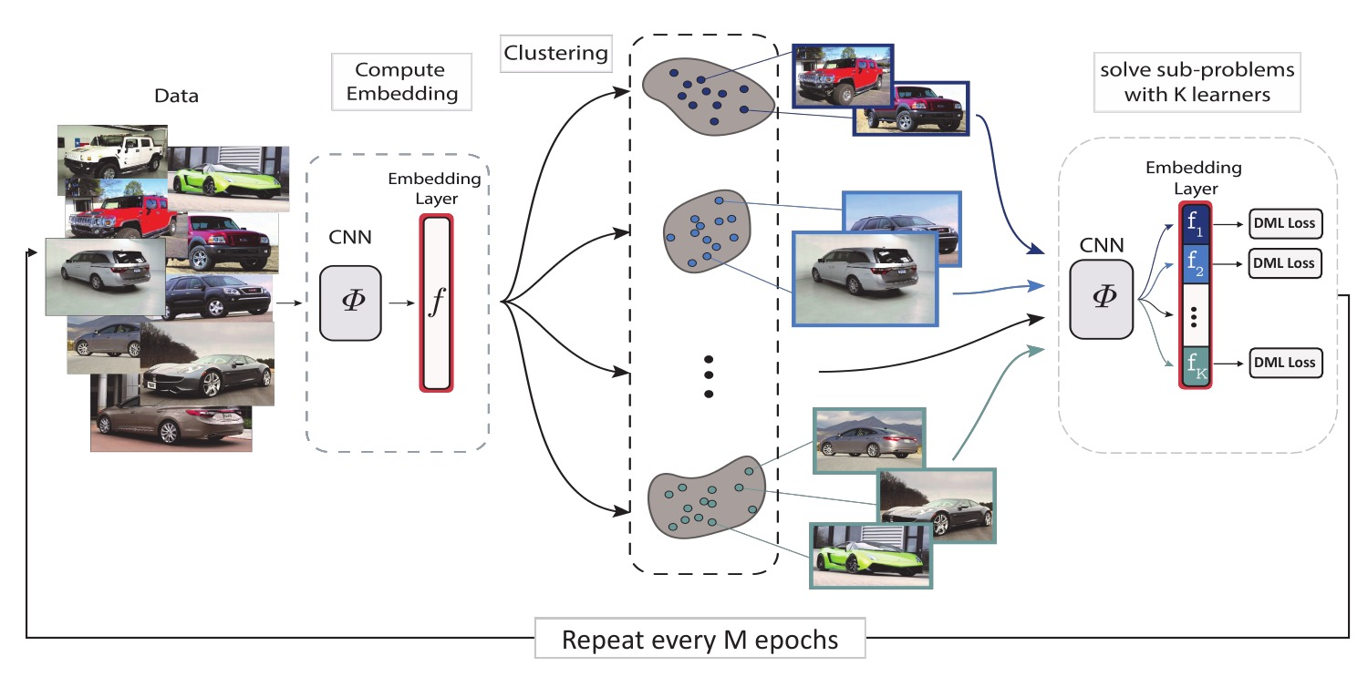
1. Compute embeddings for all train images
K clusters
2. Split the data into K disjoint subsets
Method
3. Split the embedding space in K subspaces of d/K dimensions each.
Split the embedding space in K subspaces
4. Assign a separate learner (loss) to each subspace.
Method
5. Train K different distance metrics using K learners.
K Learners
Method
6. Repeat every M epochs
Method: Summary
- Compute embeddings for all train images
- Split the data into K disjoint subsets
-
Split the embedding space in K subspaces of d/K dimensions each.
-
Assign a separate learner (loss) to each subspace.
-
Train K different distance metrics using K learners.
- Repeat steps 1-5 every M epochs
Implicit Hard-negative Mining

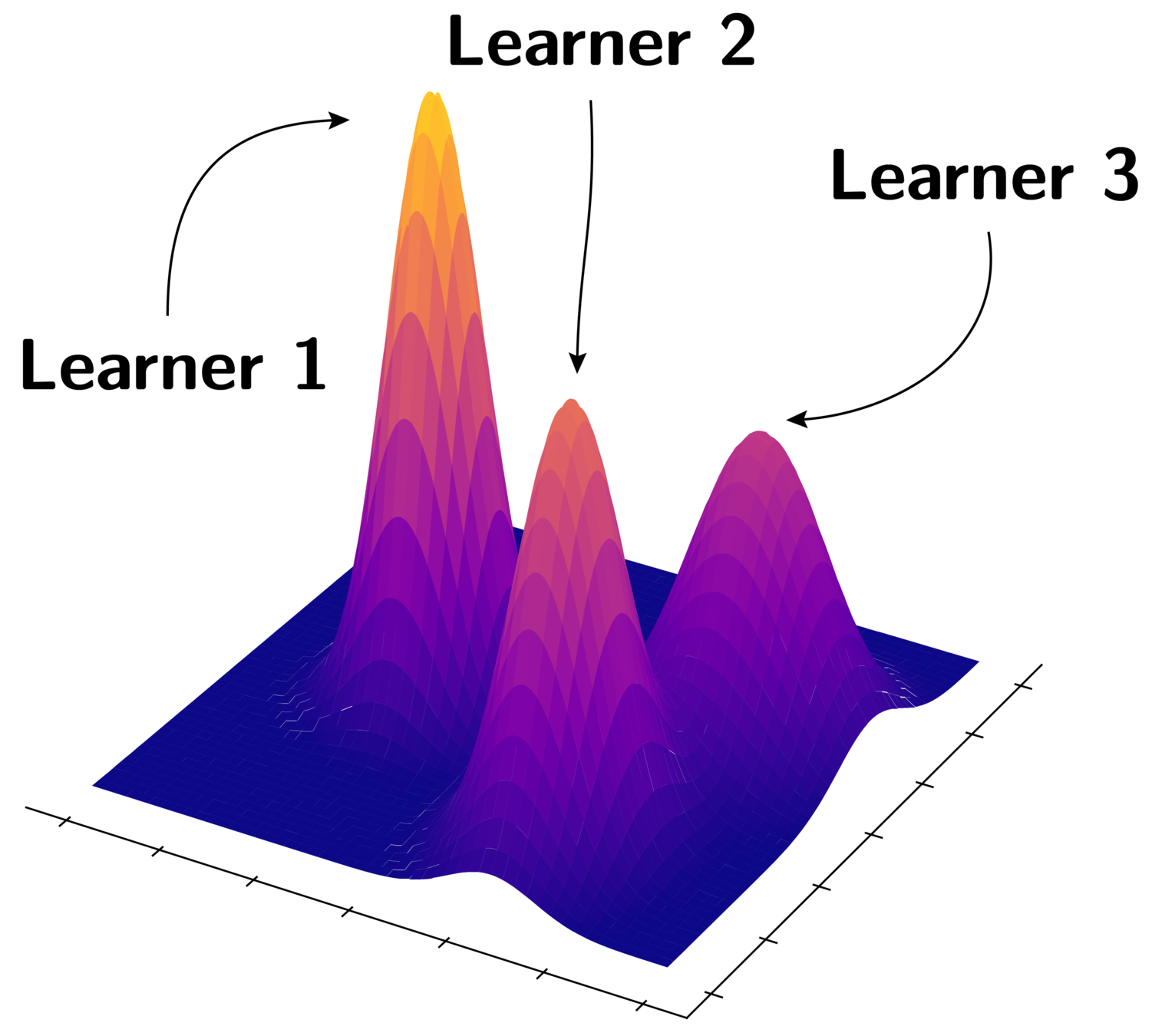
Every learner is trained on the data within one cluster
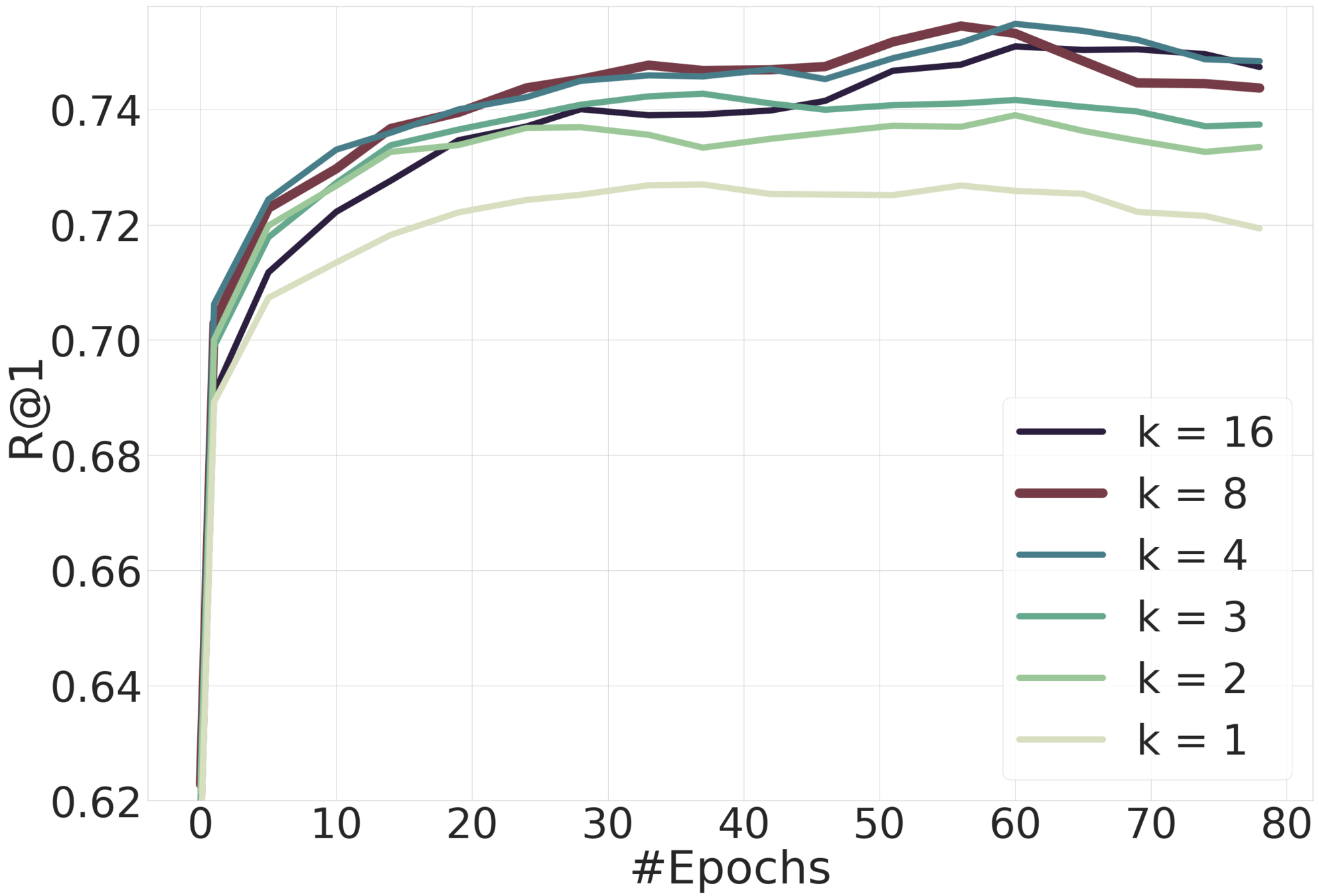
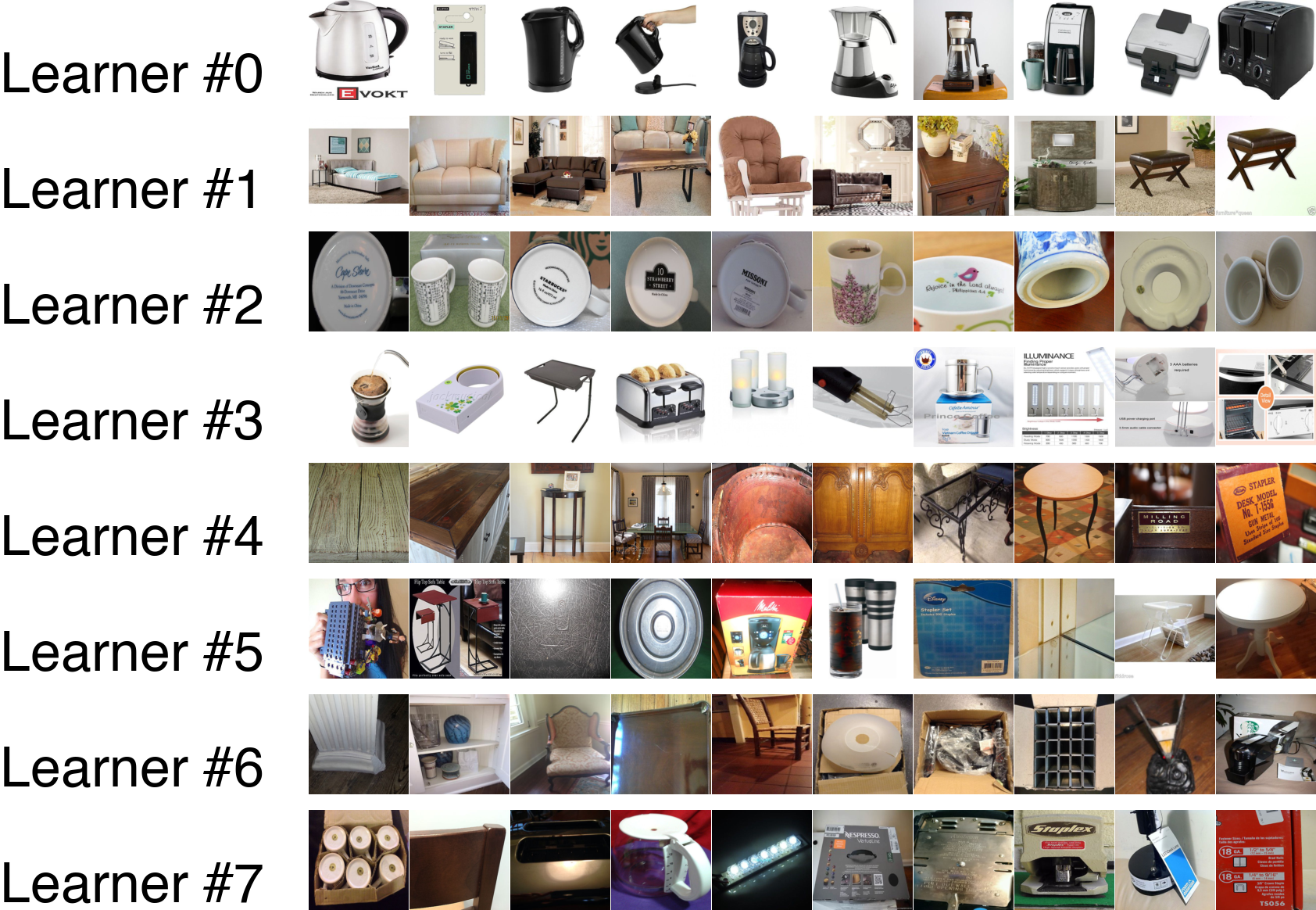
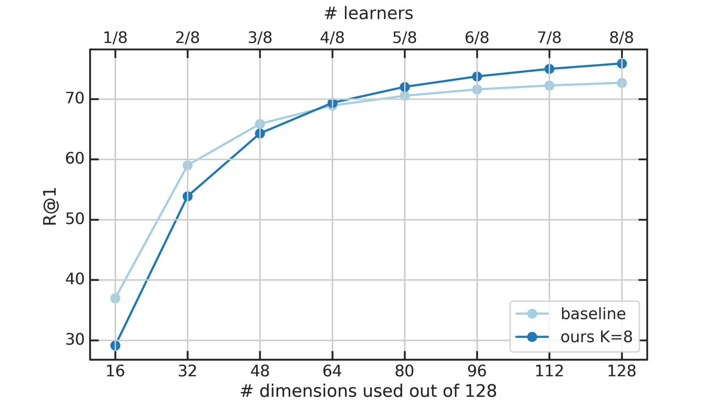
Comparison with SOTA
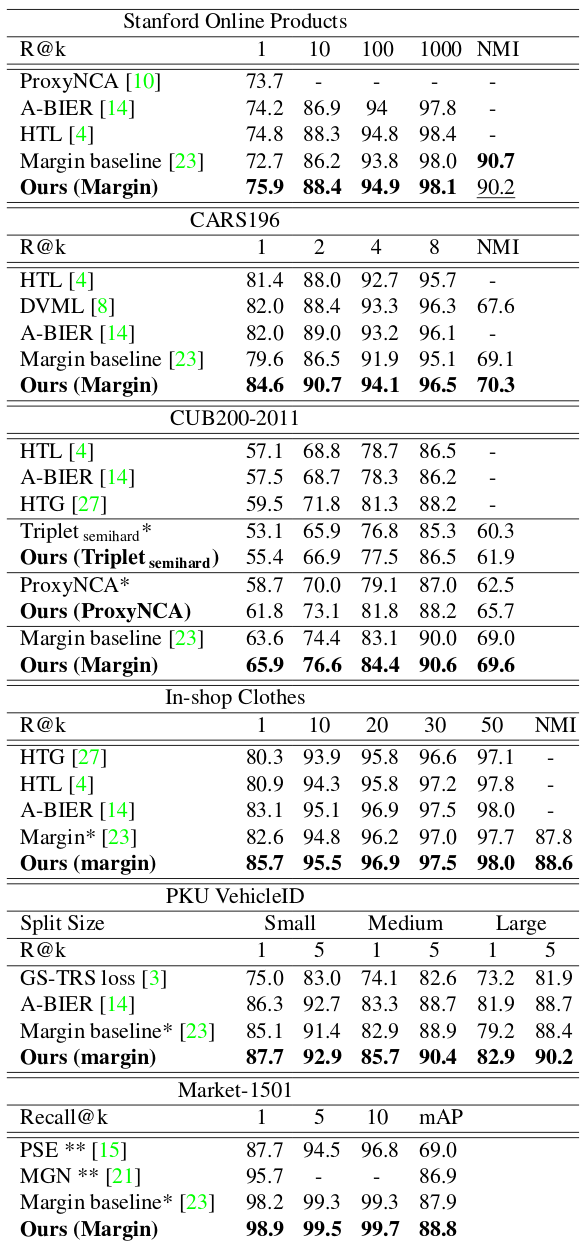
Let's Look at Learners
Qualitative results
Qualitative results
Conclusion

-
Jointly split the data into K disjoint subsets and the embedding space in K subspaces of d/K dimensions each.
Train K different distance metrics using K learners. - Does not require network architecture change
- The proposed method can be applied to any metric learning loss function.
-
Achieves state-of-the art results on 6 benchmark datasets.

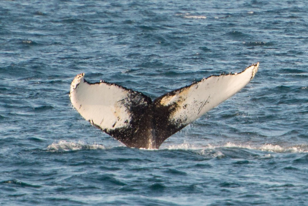
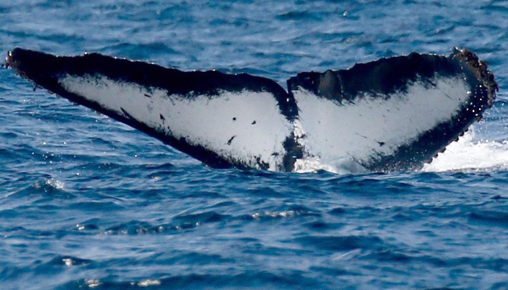
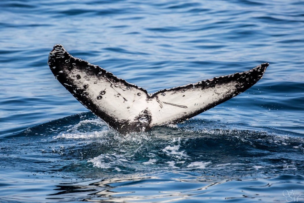
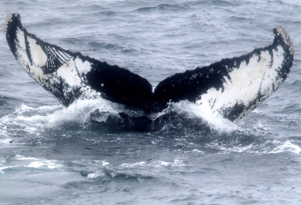
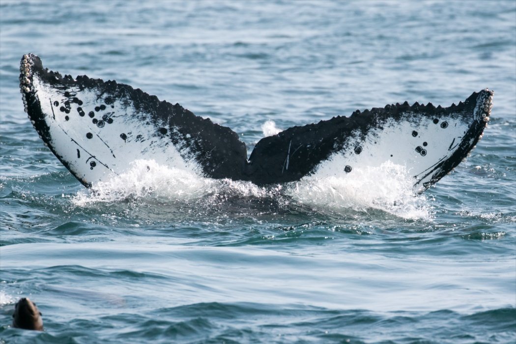
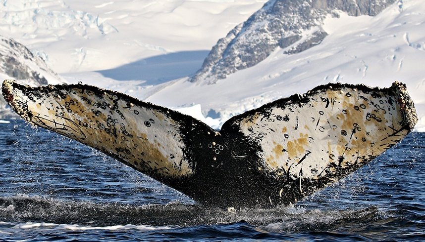
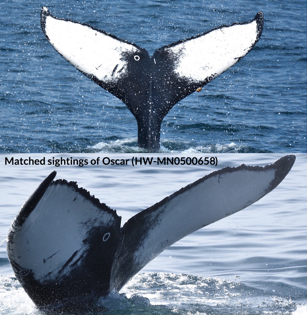
Humpback Whale Identification Challenge
Problem Overview
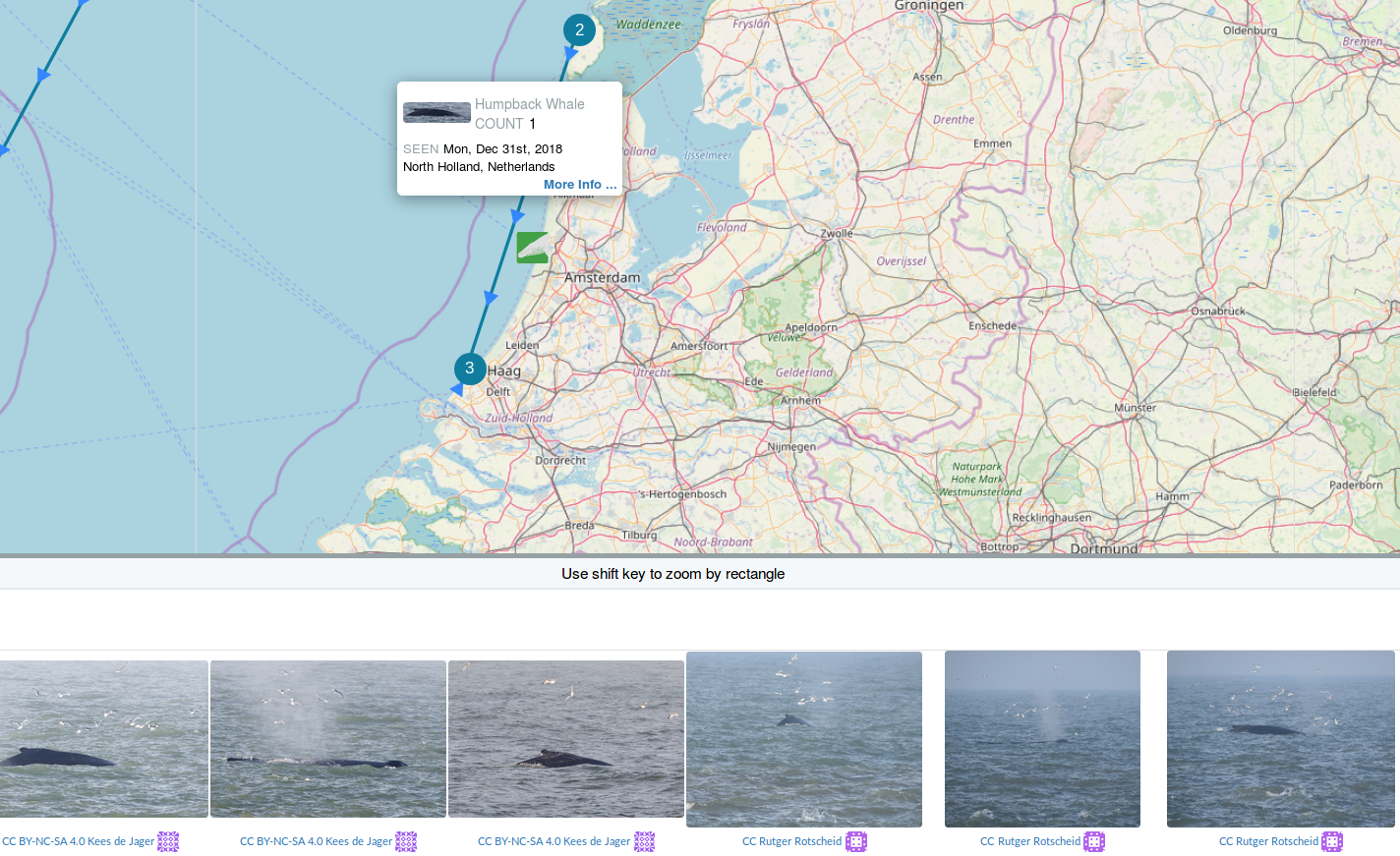
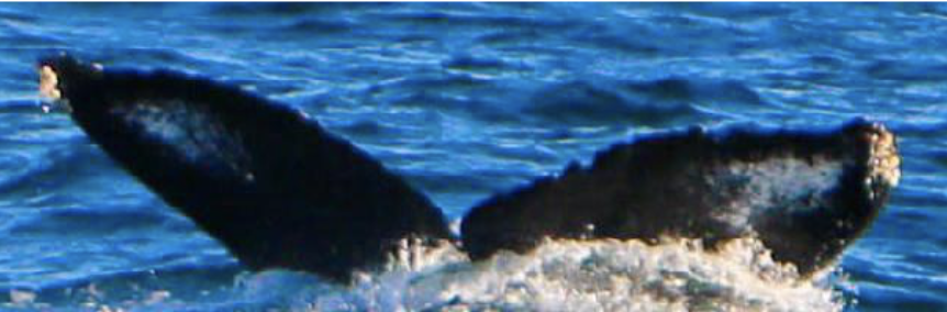
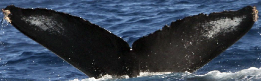
Can you identify a whale by its tail?
- 2,131 Teams
- $25,000 Prize Money
- 3 Month Time
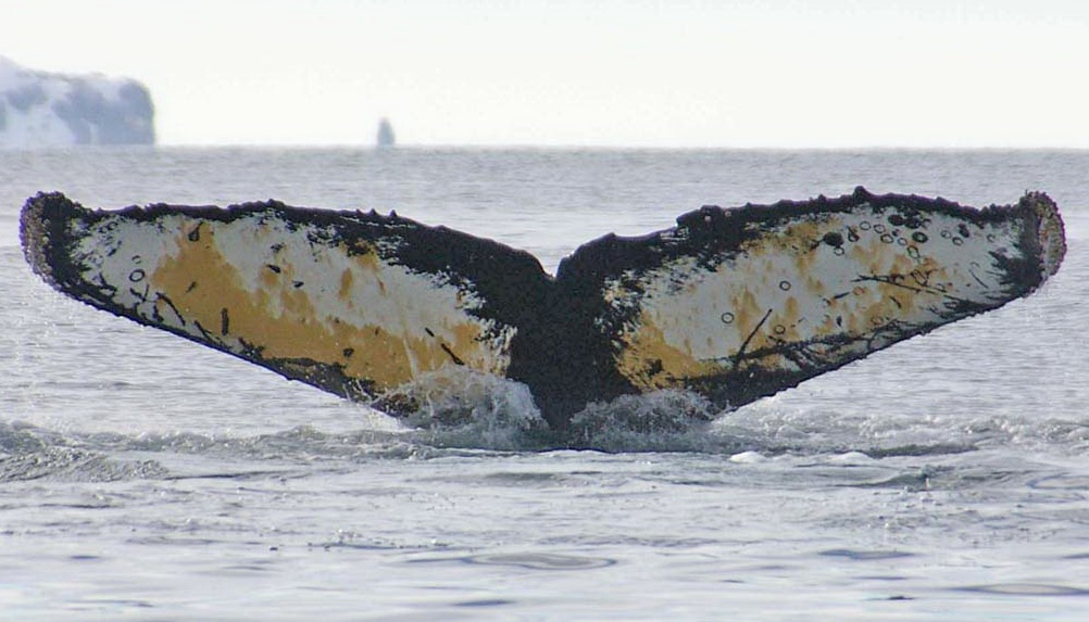
Which whale is it?
Oscar
Match!
Challenge Organizer
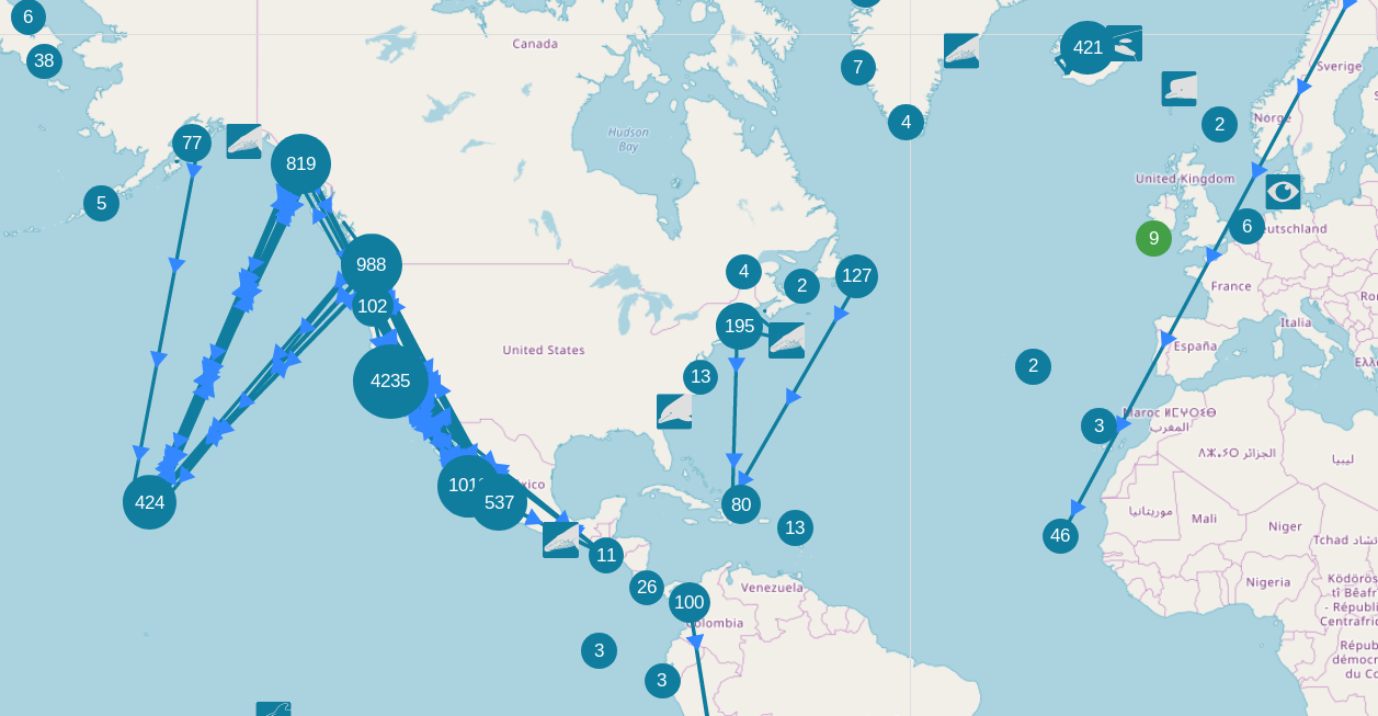
Happywhale engages citizen scientists to identify individual marine mammals, for fun and for science
They tracks your whales around the globe
Team
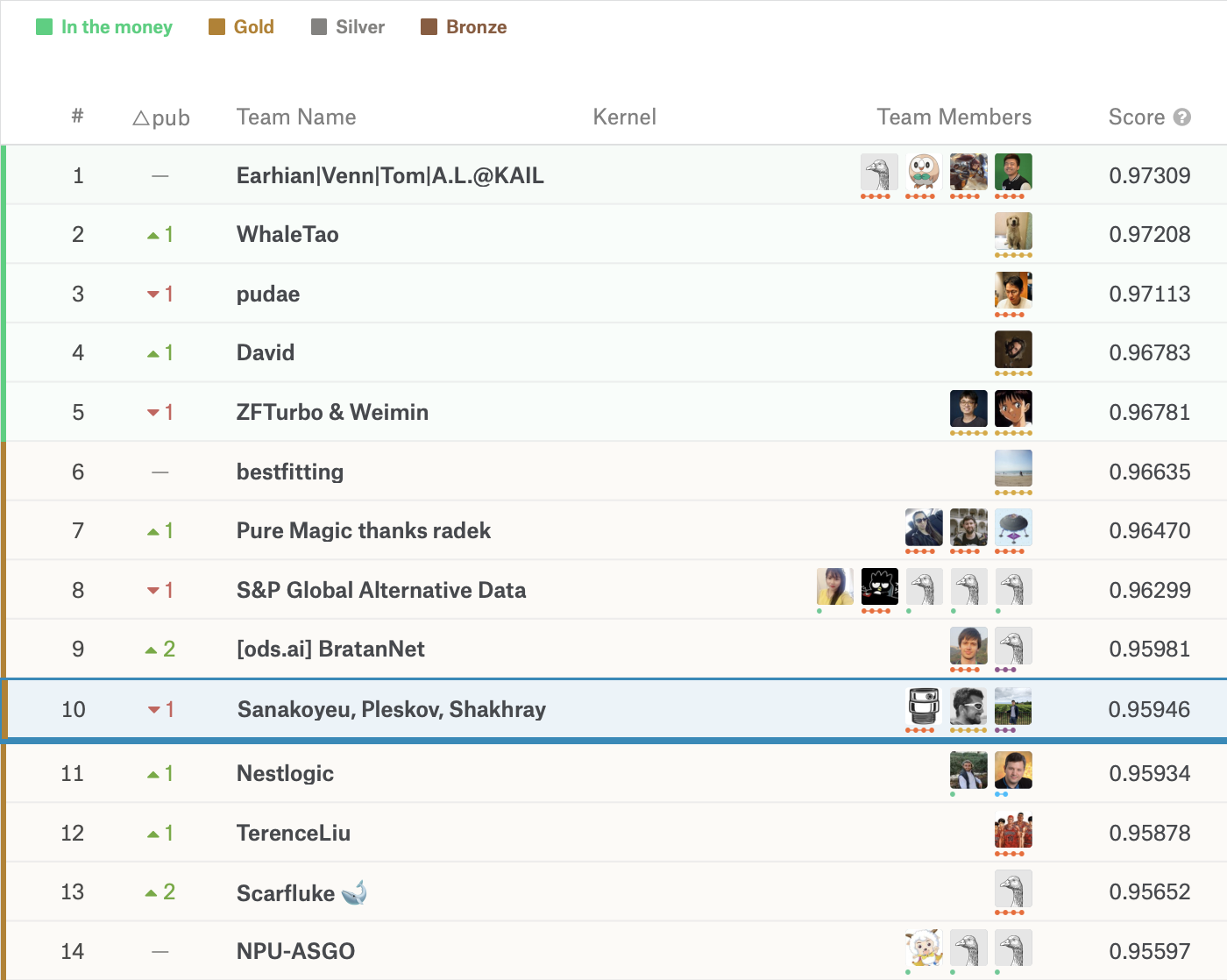
We finished #10 / 2131 Teams


Vladislav Shakhray
MIPT Student,
Russia
Artsiom Sanakoyeu
Me
Pavel Pleskov
Data Scientist at Point API
Russia
Open Data Science - Russian Speaking Data Science Community: ODS.ai
Data Overview
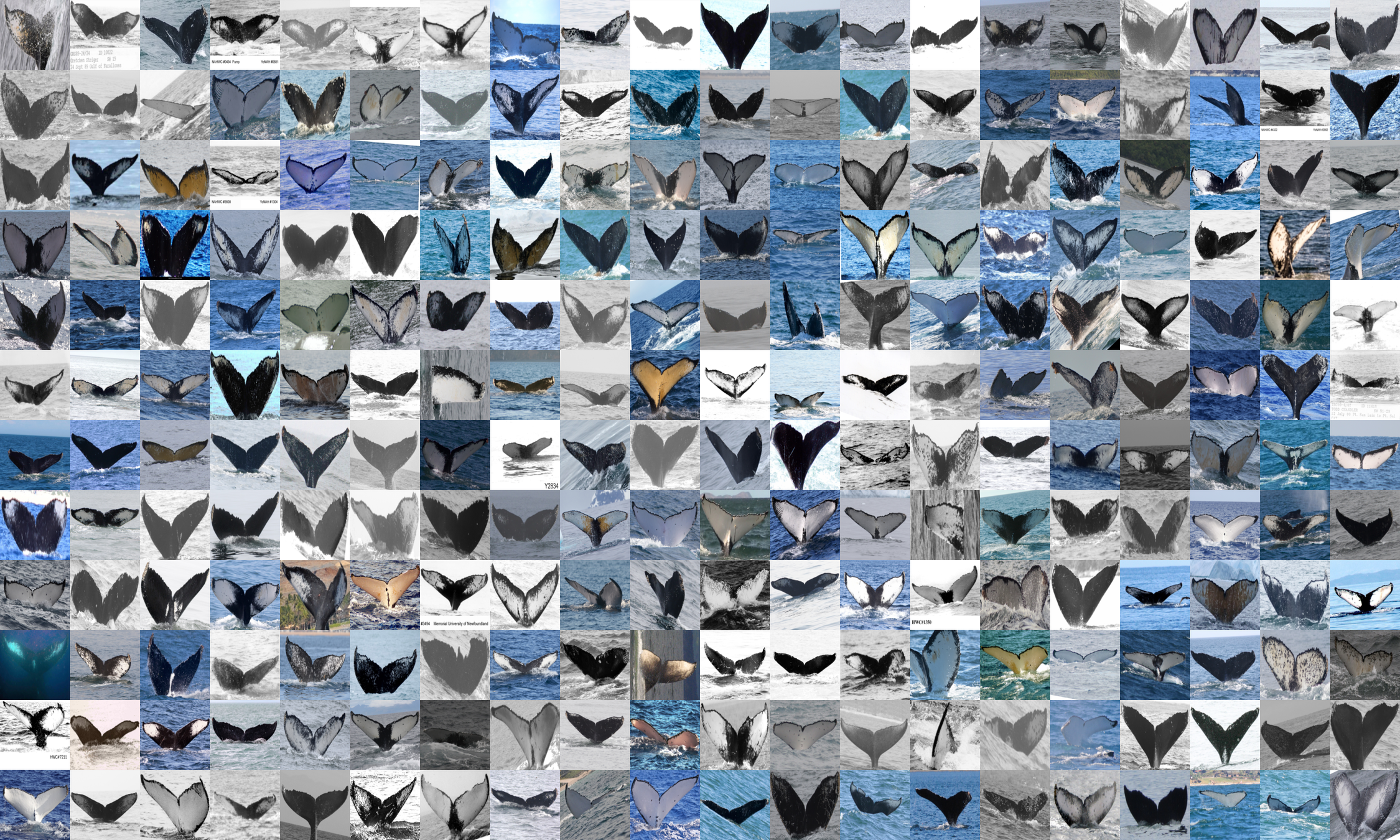
- 5004 classes
- 25.361 Train images
- 7.960 Test images
Problem Overview

Identify among 5004 whale IDs or predict "new whale"
Query image
Find a match in the train set
Other train images
- 5004 classes +
"new whale"
(yet unknown whales) -
Highly imbalanced data
- 25.361 Train images
- 7.960 Test images
- Public test / Private test = 20%/80%
Class size distribution
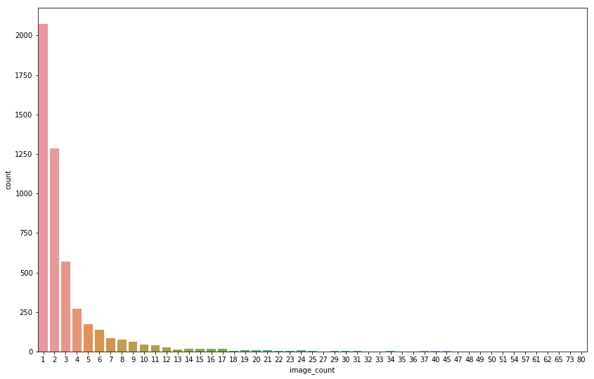
Data Overview
Evaluation Metric
Mean Average Precision @ 5
N is the number of images,
P(k) is the precision at cutoff k,
n is the number predictions per image,
rel(k) is an indicator function equaling 1 if the item at rank k is a relevant (correct) label, zero otherwise.
Validation and Preprocessing
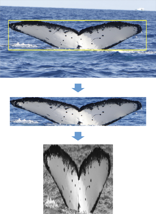
- Hold-out validation set (20% of Train)
- Remove "new whale" from train
- Train detector and detect flukes
- Crop the flukes
- Convert to black&white
- Resize to square
Typical
Step 1: More layers!
Step 2: More Different Models!
????????
Step 3: PROFIT!!!

Our Models
A. Ensemble of:
- Two-stream Siamese Networks
- Three-stream Siamese Networks
- Total: 29 networks.
B.
Softmax classifier on top of features from 29 networks.
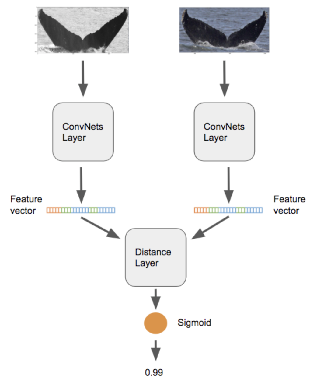
A1. Two-Stream Siamese Network
Backbones:
- ResNet-18, ResNet-34, ResNet-50
- SE-ResNeXt-50 (MAP@5=0.929)
Tricks:
- Hard-negative, hard-positive mining
- Progressive learning (299->384)
- Adam, reduce 5 times on plateau
- Batch size: 64
- Test-time augmentations (TTA)
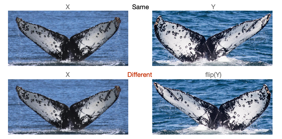
A1. Two-Stream Siamese Network: Augmentations
- Smart flipping strategy
- Gaussian noise, blur, brightness, contrast
A2. Three-Stream Siamese Network
Backbones:
- ResNet (50, 101, 152),
DenseNet (121, 169) - Best single model:
DenseNet-169 (MAP@5=0.931)
Tricks:
- Margin loss
- Progressive learning (448->672)
- Hard-negative mining
- Adam, batch size 96
- Random flips +
Color augmentations - Inference: dot product
“Divide and Conquer the Embedding Space for Metric Learning”, Sanakoyeu et al., In CVPR 2019
B. Softmax Classifier on Aggregated Features
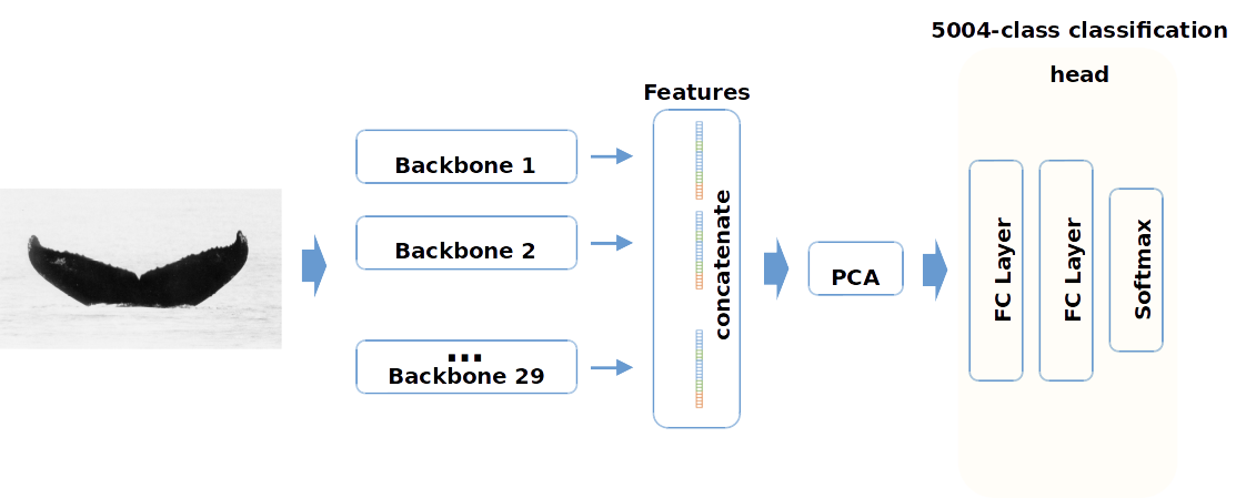
MAP@5=0.924 LB
~12.000 dim
2048 dim
B. Softmax Classifier on Aggregated Features
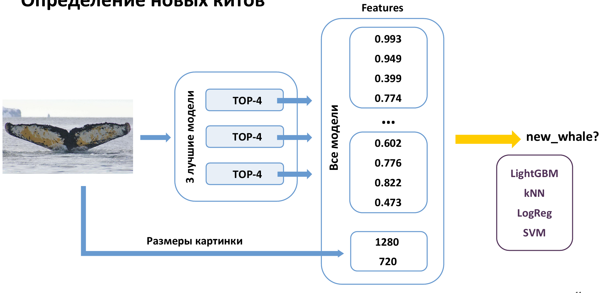
Image size
3 Best models
class probabilities
Extra Tricks
- The backbones were ImageNet-pretrained
- Pseudo-labeling (semi-supervised learning) helped:
1. Impute labels for test images using the best ensemble
2. Add test images from the previous step in train and retrain models.
Conclusion
- Finished #10 out out 2131 Teams -> Gold medal
- Final ensemble on private test: MAP@5=0.959
- Had a lot fun and polished practical skills
- Blog post: https://towardsdatascience.com/a-gold-winning-solution-review-of-kaggle-humpback-whale-identification-challenge-53b0e3ba1e84
Thank you!