Obtain original web presentation here:
https://slides.com/odineidolon/chym2019-3/fullscreen#/
This PDF version is of lower quality
Statistical analysis for flood mapping estimation
Francesca Raffaele, Rita Nogherotto, Adriano Fantini
ICTP, Trieste, Italy
afantini@ictp.it
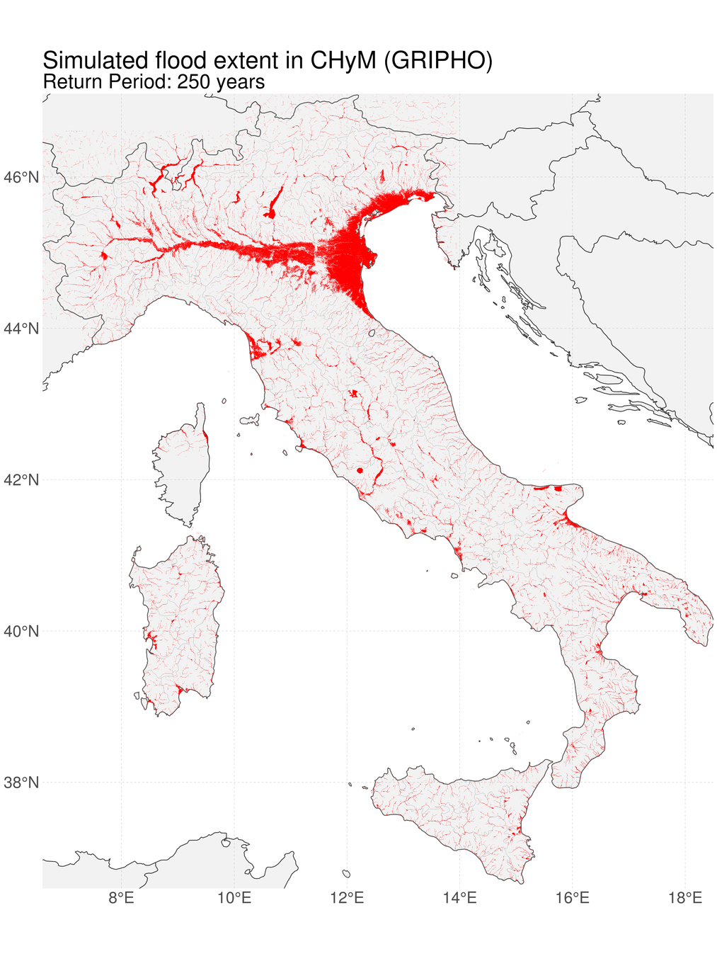
Objective:
flood hazard maps
- Different Return Periods (probabilities): 100, 200, 500 years...
- Italian territory
- Future climate projections
- Using data from hydrological model
Methodology
Precipitation:
- Observations
- RCM output
Gridded netCDF:
- River network
- Discharges
hydrological model

For each RP, cell:
- Gumbel distr.
- Hydrographs
- Extreme Q
Statistical analysis
For each RP, cell:
- Flood extent
- Flood depth
(multiple simulations)
- RCM output
- Discharges
- Floods
Validation and change for

CA2D hydraulic model
Based on Maione et al., 2003
(over nine domains)
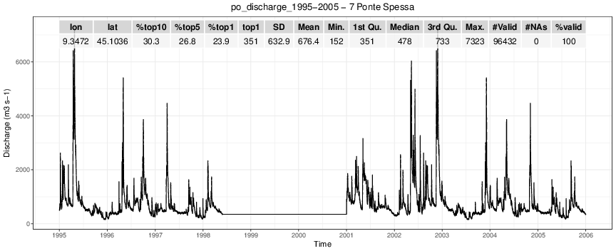
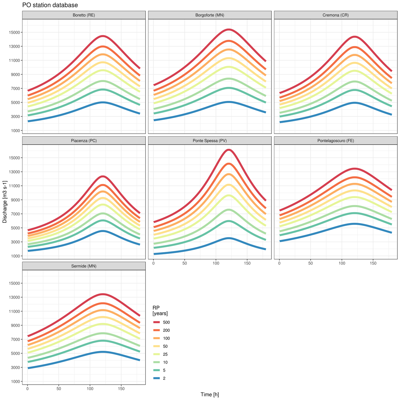
Discharge timeseries from hydrological simulation
Synthetic Design Hydrographs: "typical" flood event, input to hydraulic model
HOW?
HOW?
Basic concept (1):
Return Period
The RP is a common measure of probability used for extreme events: it represents the probability of the event happening any given year. For example:
- If an event has RP=100 yr, its probability to happen any given year is 1%
- RP=200 yr => p=0.5%
- Only a statistical measure!
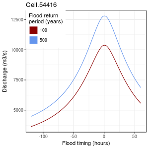
Basic concept (2):
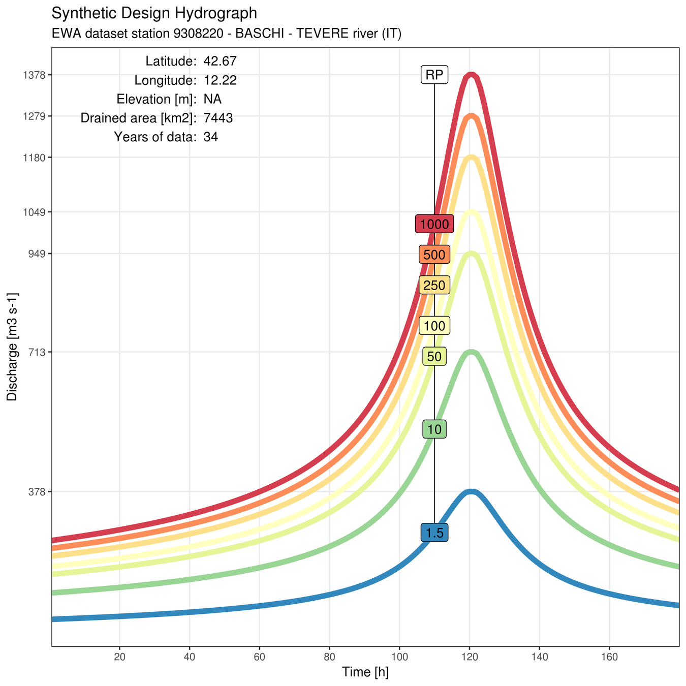
Synthetic Design Hydrographs
The SDH is the curve giving the "typical" flood event discharge (Q) as a function of time (t), for any given Return Period (RP):
There are two components to the SDH (at a given RP):
- peak discharge
- shape
Time (h)
Basic concept (3):
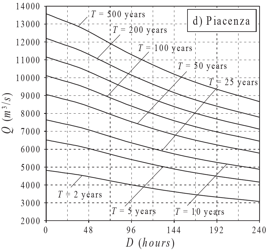
Flow Duration Frequency curve
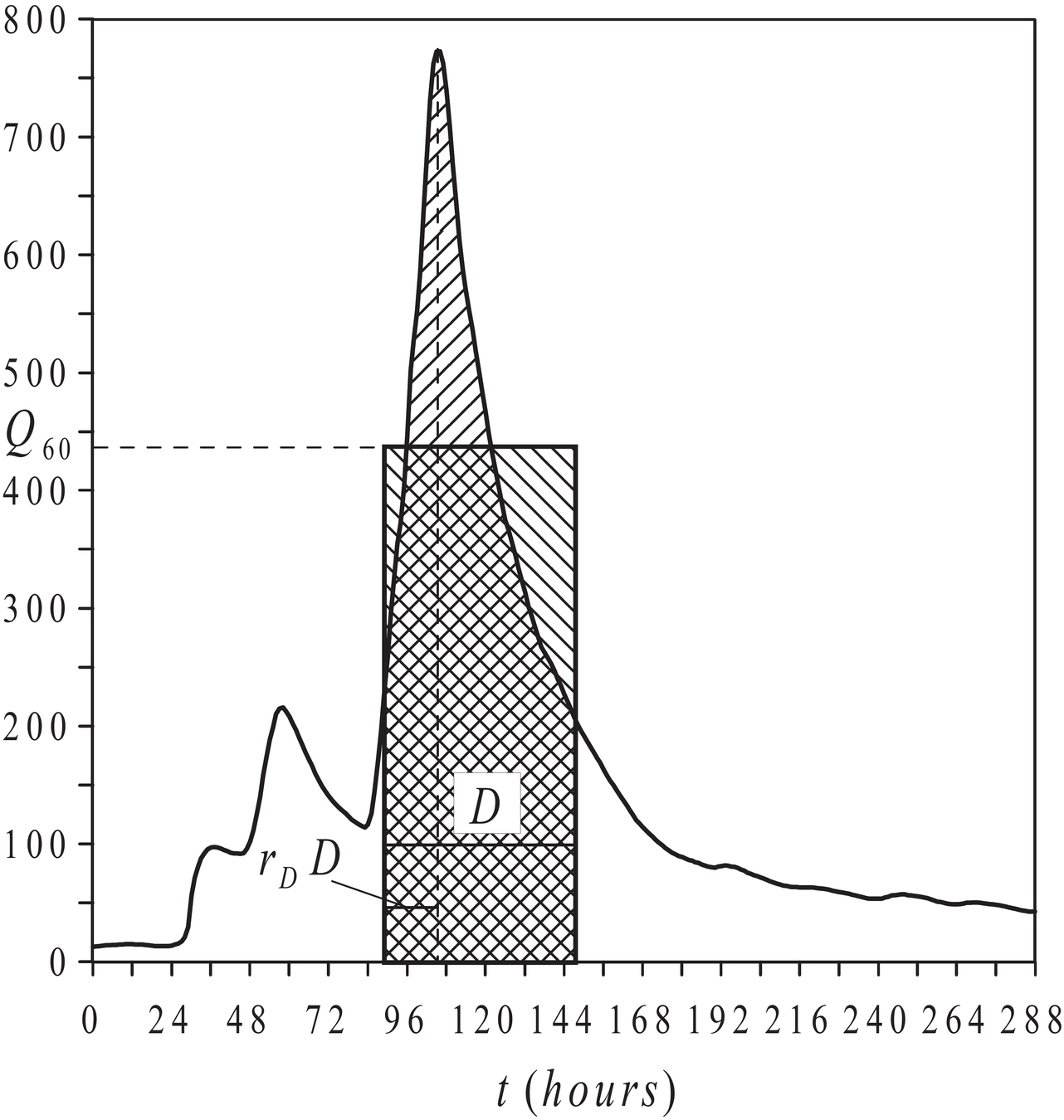
The FDF is the curve maximising the flood event discharge (Q) averaged over a duration (D) around the peak, so that for a given event:
Notice that, by definition, for an idealised event with Return Period RP, the peak flood discharge is:
Basic concept (3.1): confused?
Example time!
FLOOD PEAK
DURATION
FDF(60)
From Maione, 2003
The shape of the SDH is dictated by the peak-duration ratio , which is the ratio of the time before the peak and the total duration (D) of the averaging window.
The smaller the , the more skewed the hydrograph will be towards steeper (flatter) rising (falling) limbs of the hydrograph.
Also notice that:
Two assumptions
Following Maione et al. (2003), we assume that the reduction ratio ( ), which is the ratio of the FDF and the peak flood discharge is constant for any Return Period (RP), so that:
Which is a reasonable assumption also according to NERC (1975): the shape of the hydrograph, given by this ratio, does NOT depend on the RP!
Moreover, following Alfieri et al. (2014), we assume that the hydrograph is symmetric, that is to say that:
Step 1: split the hydrograph
Set the flood peak as t=0, and split the left and right limb of the SDH as follows:
t=0
FDF
Step 2: differentiate for D
Only for the falling limb, differentiate the previous equation with respect to D:
Where:
Once we know the reduction ratio and the FDF, we can then calculate the SDH!
But remember that we set the reduction ratio to one half, so that:
Step 3: obtain the reduction ratio
Remember:
We assume (Maione, 2003):
Where:
Where θ only depends on the (known!) drained area; a function for it is conveniently obtained by Maione based on observed data. We are only missing !
Step 4: obtain the peak discharge
Possible approach: fitting an extreme value distribution, such as a Gumbel distribution (Maione, 2003; Alfieri, 2015) to the distribution of yearly maxima:
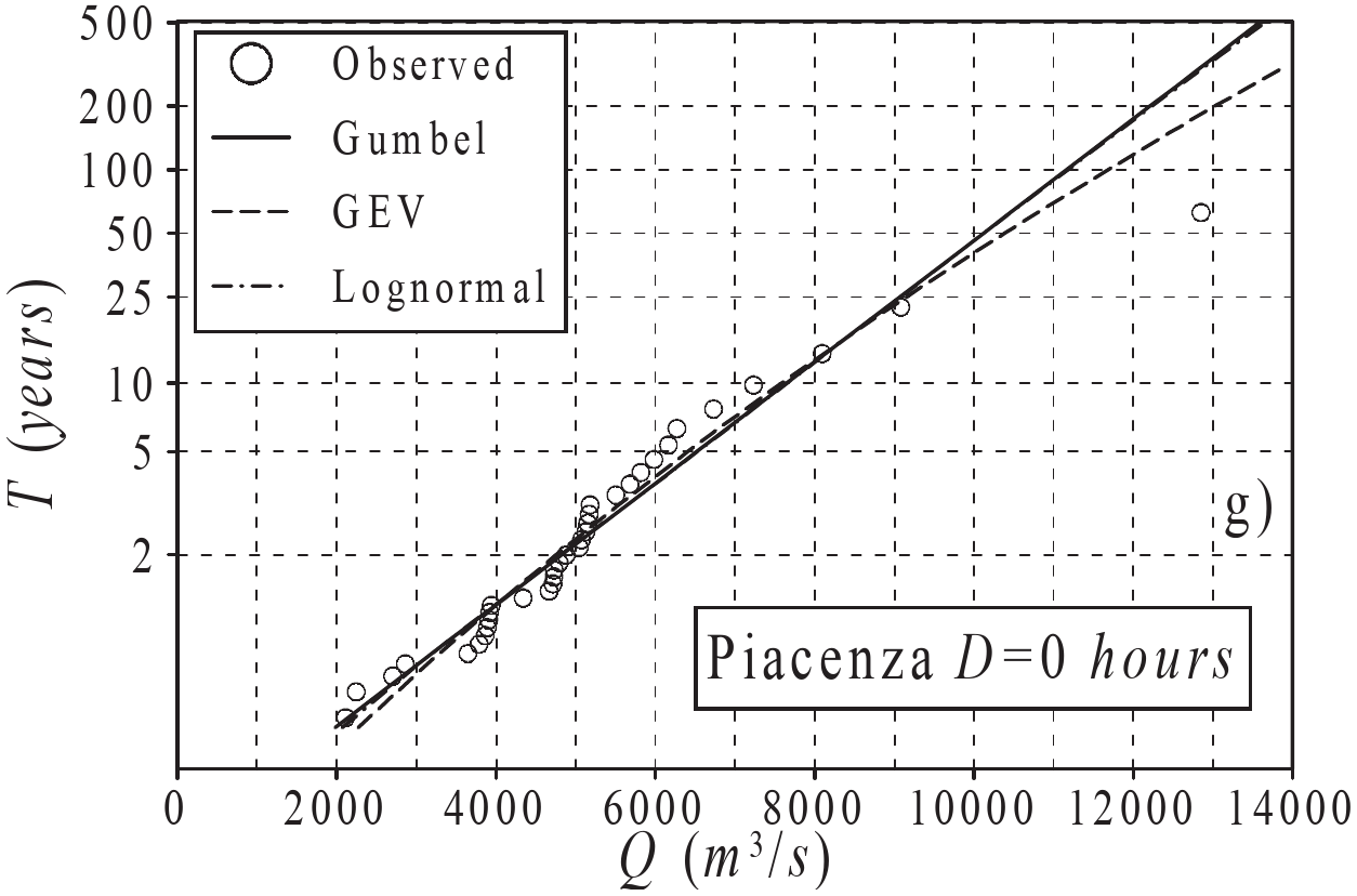
we use the available years of data (up to 30) to estimate the peak discharge for any RP, thus extrapolating data for higher Return Periods!
Now:
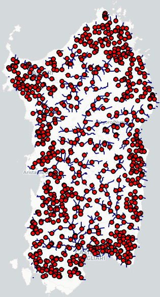
- Do this procedure for each 5-10 km along rivers
- Run 5528 hydraulic simulations
- Aggregate data...
THANK YOU!
-
Rita Nogherotto will present the results from the hydraulic model tomorrow!
-
Francesca Raffaele will be here next week to answer any question