History

Mathematical Modeling of engineering problems leads to

Ordinary differential equations
Partial differential equations
Integral equations
Optimal control

Ordinary differential equations

$$y''(x) + \frac{2}{x} y'(x) + y^m(x)=0$$

$$y(0)=1\\y'(0)=0$$

Lane-Emden equation
Describes the temperature variation of a spherical gas cloud under the mutual attraction of its molecules
Exact solution only for $m=0,1,5$.

Ordinary differential equations

A linear first order differential is defined as

with the exact solution

$$z(t) = z(t_0) + \int_{t_0}^{t_1} f(z(t),t)\ dt$$

$$\frac{{dz}}{{dt}} = f\left( {z(t),t} \right),\ \ \ z \left( {{t_0}} \right) = {z_0},$$

Solving strategies for ODEs

Analytical Methods
- Separation of variables
- Laplace transform
Numerical Methods
- Finite differences
  - Euler method
  - Runge-kutta
  - Adams–Bashforth

Euler method for ODEs

Introduced at 1880s.
The most basic method for approximating ODEs
An explicit method
A single-step method

Euler method for ODEs

can be approximated by

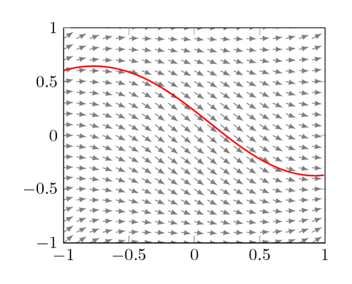
Theorem. The solution to the following IVP

where $\Delta t = t_n- t_{n-1}$ is an small step-size.

$$\frac{{dz}}{{dt}} = f\left( {z(t),t} \right),\ \ \ z \left( {{t_0}} \right) = {z_0},$$

$${z_{n + 1}} = {z_n} + \Delta t\,{f(z_n, t_n)},\quad n=1,2,\ldots$$

Modern ODE solvers

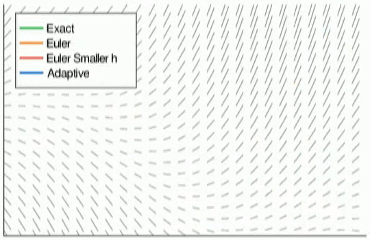
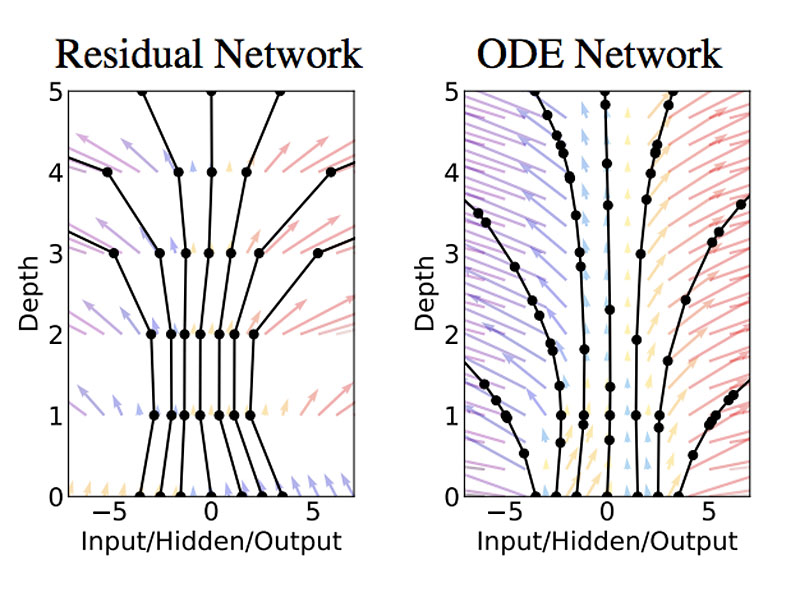
Euler method vs. modern solvers

Deep Neural Networks

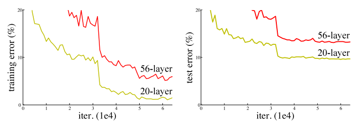
Training error (left) and test error (right) on CIFAR-10 with 20-layer and 56-layer “plain” networks.

Residual Neural Networks

Overcome vanishing gradient by skip connections
Learn the residual function
Much more powerful than traditional networks in most cases

He, Kaiming, Xiangyu Zhang, Shaoqing Ren, and Jian Sun. "Deep residual learning for image recognition." In Proceedings of the IEEE conference on computer vision and pattern recognition, pp. 770-778. 2016.

Skip connection

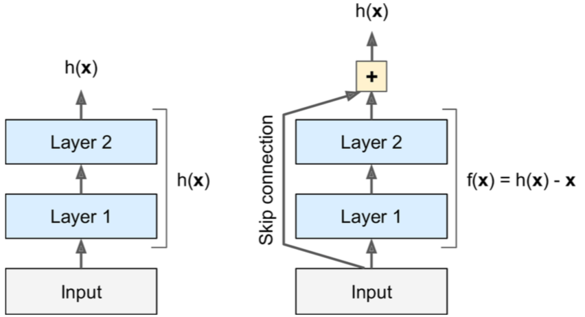
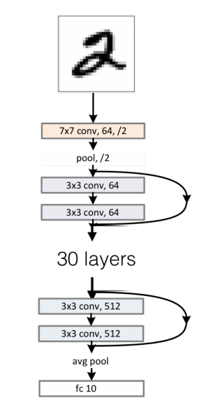
Traditional networks vs Resnets

Residual Neural Networks

In a general form, ResNets can be formulated as

\begin{aligned} y_t &= h(z_t) + \mathcal{F}(z_t,\theta_t)\\ z_{t+1} &= f(y_t) \end{aligned}

$\mathcal{F}(.)$ is a simple neural network (Residual block )
$f, h$ are element wise functions such as ReLU
$\theta_t$ is the unknown weight for layer $t$
$z_t$ is the output of layer $t$

Residual Neural Networks

By setting functions $f,h$ as identity mappings

we can see a relation between ResNets and Euler method!

$$z_{t+1} = z_t + \mathcal{F}(z_t, \theta_t)\\$$

Residual Neural Networks

A chain of residual blocks in a neural network is basically a solution of the ODE with the Euler method!

NNs as ODE solvers

Network	Fixed-step Numerical Scheme
ResNet, RevNet, ResNeXt, etc.	Forward Euler
PolyNet	Approximation to Backward Euler
FractalNet	Runge-Kutta
DenseNet	Runge-Kutta

New Idea

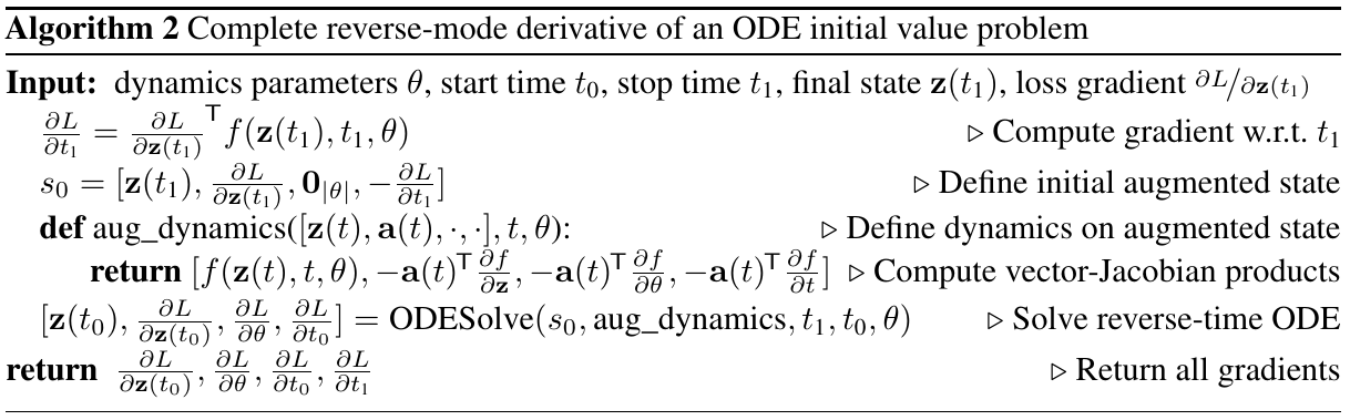
Let’s replace ResNet / EulerSolverNet with some abstract concept as ODESolveNet with much better accuracy than Euler’s method

Neural Ordinary Differential Equations

Chen, Tian Qi, Yulia Rubanova, Jesse Bettencourt, and David K. Duvenaud. "Neural ordinary differential equations." In Advances in neural information processing systems, pp. 6571-6583. 2018.

One of the best research papers of NeurIPS 2018
Presents a continuous model
Solves the ODE with a black-box ODE solver

Neural Ordinary Differential Equations

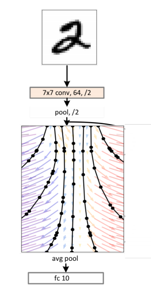
Predict the output value for input $x$ by solving $$\frac{{dz}}{{dt}} = \mathcal{F}\left( {z(t),t,\theta} \right)$$ w.r.t initial condition $$z \left( {{0}} \right) = {x},$$ by a black-box ODE solver where $$t \in [0, T].$$

Neural Ordinary Differential Equations

Left: A Residual network defines a discrete sequence of finite transformations.
Right: A ODE network defines a vector field, which continuously transforms the state.
Circles represent function evaluation locations.

The effect of adaptive solver

NODE: Benefits

Adaptive computation
Memory efficiency
Parameter efficiency
Continuous time-series models
Error Control

NODE: Continuous model

def F(z, t, θ):
    return nnet([z,t], θ)

def FixedNODE(z):
    for t in [1:T]:
        z = z + F(z, t, θ)
    return z

def F(z, t, θ):
    return nnet([z,t], θ)

def AdaptiveNODE(z):
    z = ODESolve(F, z, 0, T, θ)
    return z

def F(z, t, θ):
    return nnet(z, θ[t])

def resnet(z):
    for t in [1:T]:
        z = z + F(z, t, θ)
    return z

def F(z, t, θ):
    return nnet[t](z, θ[t])

def resnet(z):
    for t in [1:T]:
        z = z + F(z, t, θ)
    return z

Different Res Blocks for each time step

Different weights for similar Res Blocks

Shared weights, continuous model

Replace Euler with adaptive solver

NODE: Optimizing the model

$$L(z(t_n)) = L(\ z(t_0) + \int_{t_0}^{t_n} \mathcal{F}(z(t),t, \theta)dt\ )$$

$$=L(ODESolve(\mathcal{F},z(t_0),t_0,t_n,\theta))$$

$$\frac{\partial L}{\partial z(t)},\frac{\partial L}{\partial \theta}=??$$

NODE: Error Backpropagation

Naive approach: Backprop through the solver

Memory-intensive
Numerical Error

New approach: Adjoint sensitivity analysis

Approximate the derivative, don’t differentiate the approximation!
O(1) memory in backward pass!
Needs some function evaluations in backward pass

Adjoint method: linear case

Given matrices $A,C$ and vector $u$
compute $u^TB$ such that $AB=C$
Instead solve $v^TC$ such that $A^Tv = u$
proof:

$$v^TC=v^TAB=(A^Tv)^TB=u^TB$$

Adjoint sensitivity method

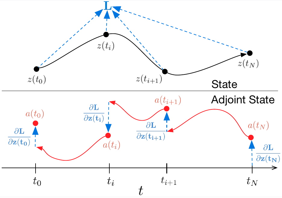
Reverse-mode differentiation of an ODE solution

Adjoint sensitivity method

Theorem. By defining adjoint state $$a(t) = \frac{\partial L}{\partial z(t)},$$ its dynamics are given by ODE

$$\frac{\text{d}a(t)}{\text{d}t} = - a(t)^T \frac{\partial \mathcal{F}(z(t),t,\theta)}{\partial z}.$$

A simple proof is available in Appendix B.

Adjoint sensitivity method

$$\frac{\partial L}{\partial t_n} = a(t_n)^T\mathcal{F}(z(t),t,\theta)$$

$$\frac{\partial L}{\partial \theta} = -\int_{t_n}^{t_0} a(t)^T \frac{\partial \mathcal{F}(z(t),t,\theta)}{\partial \theta}dt$$

$$\frac{\partial L}{\partial t_0} = a(t_n)-\int_{t_n}^{t_0} a(t)^T \frac{\partial \mathcal{F}(z(t),t,\theta)}{\partial t}dt$$

$$\frac{\partial L}{\partial z(t_0)} = a(t_n) -\int_{t_n}^{t_0} a(t)^T \frac{\partial \mathcal{F}(z(t),t,\theta)}{\partial z(t)}dt$$

All of integrals can be computed by solving an augmented ODE

Adjoint sensitivity method

In English: Solve the original ODE and the accumulated gradients backward through time.

Adjoint sensitivity method

$a = \frac{\partial L}{\partial z_t}$

$z_{t+h} = z_t + h \mathcal{F}(z_t)$

$a_t = a_{t+h} + h a_{t+h} \frac{\partial \mathcal{F}(z_t)}{\partial z_t}$

$\frac{\partial L}{\partial \theta} = h a_{t+h} \frac{\partial \mathcal{F}(z(t),\theta)}{\partial \theta}$

$a(t) = \frac{\partial L}{\partial z(t)}$

$z(t+h) = z(t) + \int_t^{t+h}\mathcal{F}(z(t))dt$

$a(t) = a(t+h) + \int_{t+h}^t a(t)^T \frac{\partial \mathcal{F}(z(t))}{\partial z(t)}dt$

$\frac{\partial L}{\partial \theta} = \int_t^{t+h} a(t)^T \frac{\partial \mathcal{F}(z(t),\theta)}{\partial \theta}dt$

Define

Forward

Backward

Params

ResNet

NODE

How deep are NODEs?

No fixed number of layers
Number of evaluations in NODEs ≈ Depth in ResNets
Dynamics become more demanding to compute during training
Regularization

Reverse versus Forward Cost

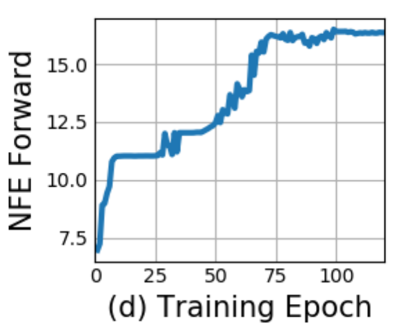
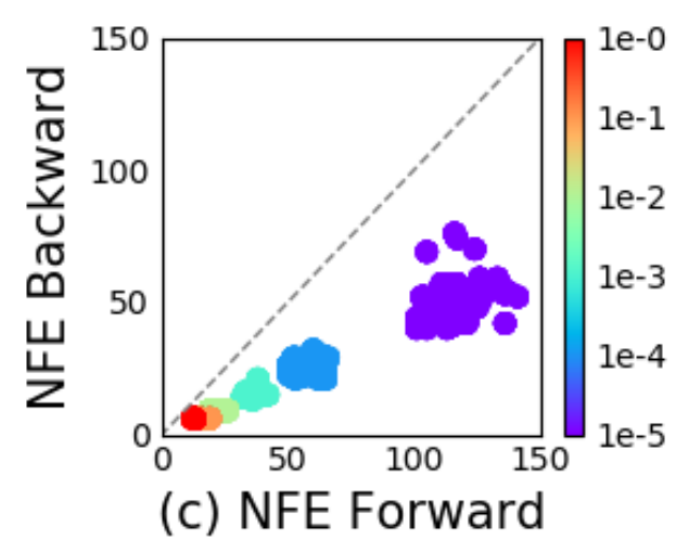
NFE = Number of Function Evaluations

Empirically, reverse pass roughly half as expensive as forward pass!
NFE can be viewed as number of layers in neural nets

NODE: implementation

Official repository in Pytorch
Non-official repository in Tensorflow, Keras and Julia

nn = Network(
  Dense(...), # making some primary embedding
  ODESolve(...), # "infinite-layer neural network"
  Dense(...) # output layer
)

Pseudocode of NODE usage

Benchmarks

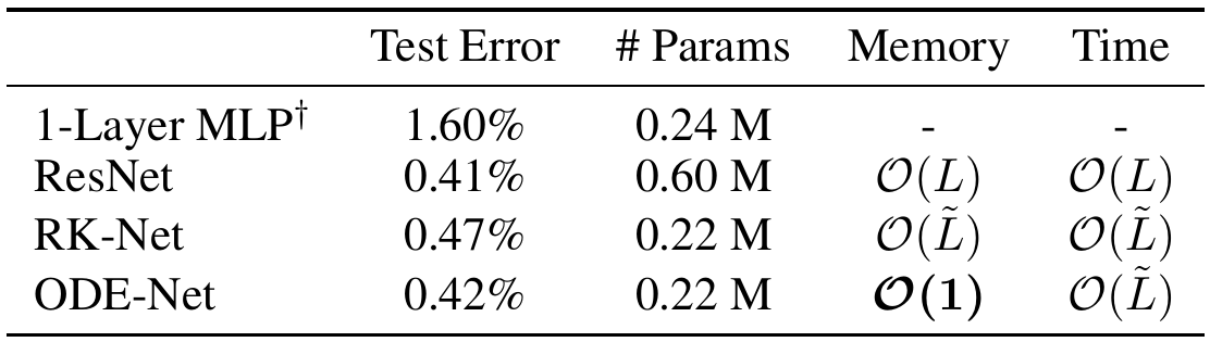
Performance on the MNIST dataset

ResNet vs NODE

Benchmarks

Model	Test score	# Params	Time (sec)
Resnet(6)	85.43%	0.6M	3700
Resnet(1)	83.62%	0.22M	1500
NODE	83.90%	0.22M	11000

Results on CIFAR-10 dataset

Benchmarks

Limitations

Mini-batching
Uniqueness
Setting tolerances
Slower than ResNets

Augmented NODEs

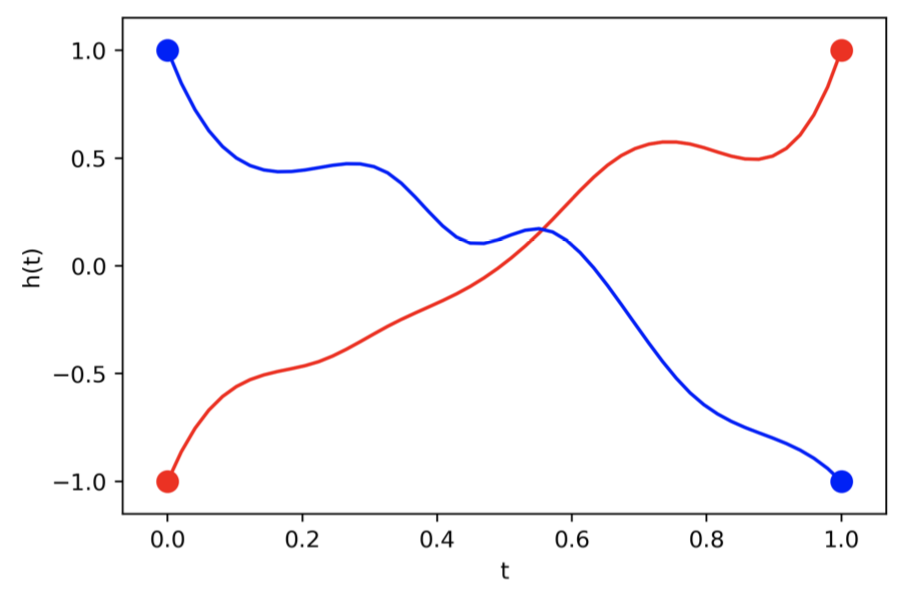
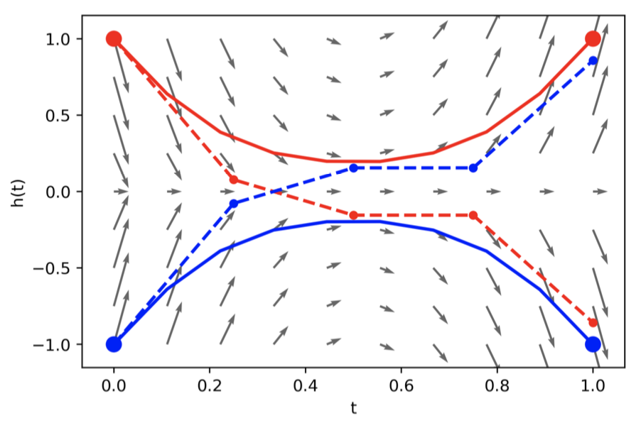
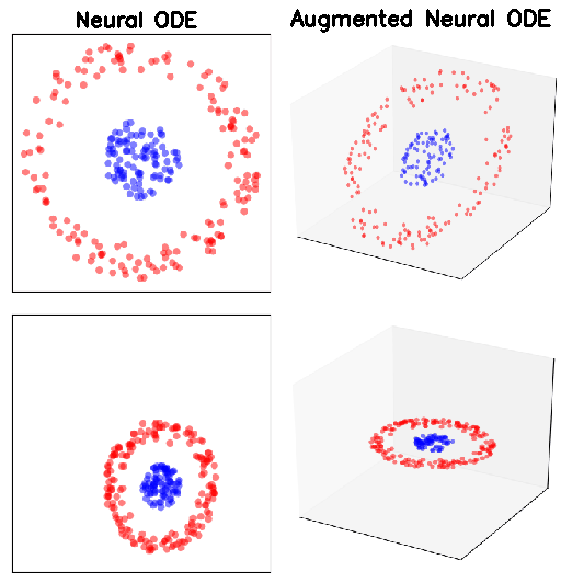
what if the map we are trying to model cannot be described by a vector field?

Ideal mapping

ResNet vs NODE

Augmented NODEs

what if the map we are trying to model cannot be described by a vector field?

Augmented NODEs

Idea: solve the problem in higher dimensional space
If our hidden state is a vector in $\mathbb{R}^n$, we can add on $d$ extra dimensions and solve the ODE in $\mathbb{R}^{n+d}$

ANODEs: Computational Cost

NFEs increase much faster for NODEs than ANODEs, presumably because ANODEs learn simpler flows

ANODEs: Image datasets

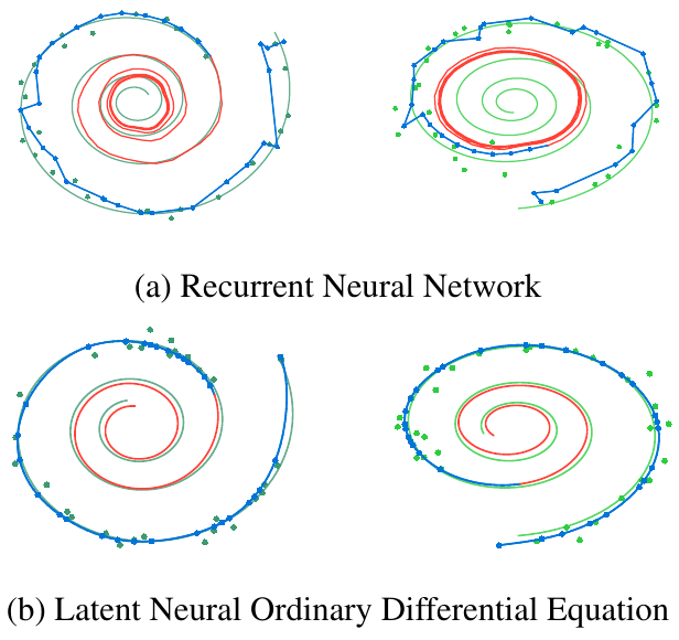
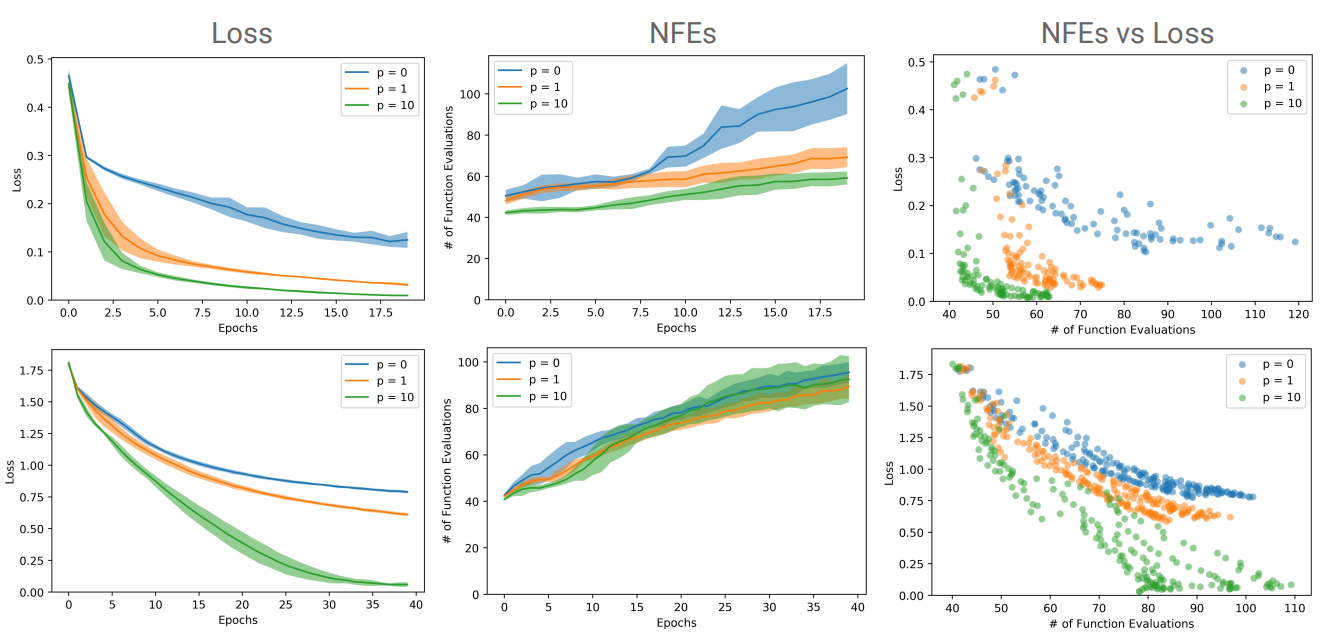
MNIST (top row) and CIFAR10 (bottom row). p indicates the size of the augmented dimension

ANODEs: Image datasets

Accuracy

ANODEs: Stability

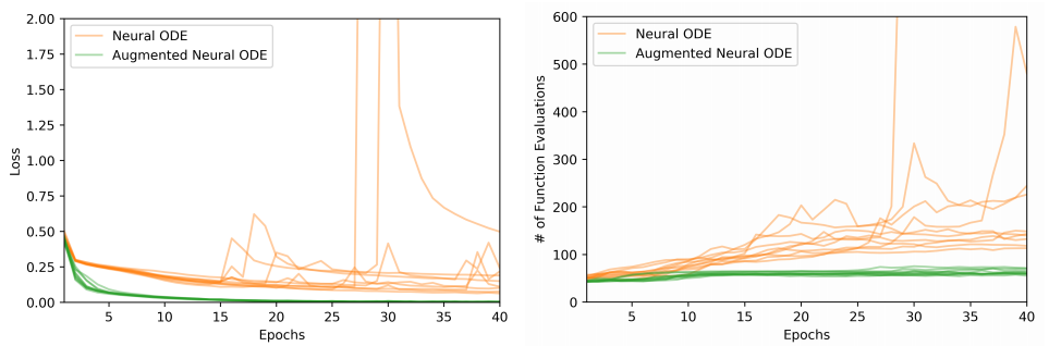
Instabilities in the loss (left) and NFEs (right) on MNIST

Implementation

$ pip install torchdiffeq
$ git clone https://github.com/EmilienDupont/augmented-neural-odes

Install the packages

import torch
import seaborn
import matplotlib.pyplot as plt

from torchvision import datasets
from torchvision import transforms
from torch.utils.data import TensorDataset, DataLoader

from anode.conv_models import ConvODENet
from anode.models import ODENet
from anode.training import Trainer

from sklearn.datasets import load_iris

Import required packages

Implementation

hidden_dim = 10
augment_dim = 10
epochs = 20

device = torch.device('cpu')

Set some variables

Load the IRIS dataset

features, labels = load_iris(return_X_y=True)

iris = TensorDataset(torch.FloatTensor(features),
                     torch.LongTensor(labels))

train_loader = DataLoader(iris, shuffle=True, batch_size=16)

Implementation

node = ODENet(device,
              data_dim=4, 
              hidden_dim=hidden_dim,
              output_dim=3,
              augment_dim=0)

optimizer = torch.optim.Adam(node.parameters(), lr=1e-3)

trainer = Trainer(node, optimizer, device,
                  classification=True, verbose=False)

trainer.train(train_loader, num_epochs=epochs)

Train a Neural ODE

Implementation

node = ODENet(device,
              data_dim=4, 
              hidden_dim=hidden_dim,
              output_dim=3,
              augment_dim=0,
              time_dependent=True)

optimizer = torch.optim.Adam(node.parameters(), lr=1e-3)

trainer = Trainer(node, optimizer, device,
                  classification=True, verbose=False)

trainer.train(train_loader, num_epochs=epochs)

Train a time-dependent Neural ODE

Implementation

anode = ODENet(device,
              data_dim=4, 
              hidden_dim=hidden_dim,
              output_dim=3,
              augment_dim=augment_dim
             )

optimizer = torch.optim.Adam(anode.parameters(), lr=1e-3)

trainer = Trainer(anode, optimizer, device,
                  classification=True, verbose=False)

trainer.train(train_loader, num_epochs=epochs)

Train an Augmented Neural ODE

Implementation

anode = ODENet(device,
              data_dim=4, 
              hidden_dim=hidden_dim,
              output_dim=3,
              augment_dim=augment_dim,
              time_dependent=True
             )

optimizer = torch.optim.Adam(anode.parameters(), lr=1e-3)

trainer = Trainer(anode, optimizer, device,
                  classification=True, verbose=False)

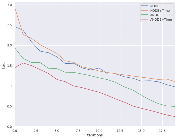
trainer.train(train_loader, num_epochs=epochs)

Train a time-dependent Augmented Neural ODE

Implementation

Comparison of models

Implementation: ConvNet

batch_size = 256
n_classes = 10
train_loader = DataLoader(datasets.MNIST('.', train=True,
                          download=True,
                          transform=transforms.Compose([transforms.ToTensor(),
                          transforms.Normalize((0.0, ), (1.0, ))])),
                          batch_size=batch_size, shuffle=True)
test_loader = DataLoader(datasets.MNIST('.', train=False,
                         transform=transforms.Compose([transforms.ToTensor(),
                         transforms.Normalize((0.0, ), (1.0, ))])),
                         batch_size=batch_size, shuffle=True)


anode = ConvODENet(device, img_size=(1, 28, 28), num_filters=16,
                   output_dim=n_classes, augment_dim=5)
optimizer = torch.optim.Adam(anode.parameters(), lr=0.001)
trainer = Trainer(anode, optimizer, device, classification=True)
trainer.train(train_loader, num_epochs=50)

What’s next?

Graph Neural Ordinary Differential Equations
Deep Neural Networks Motivated by Partial Differential Equations
PDE-Net 2.0: Learning PDEs from data with a numeric-symbolic hybrid deep network
A mean-field optimal control formulation of deep learning
Deep learning theory review: An optimal control and dynamical systems perspective
Convolutional neural networks combined with runge-kutta methods
Neupde: Neural network based ordinary and partial differential equations for modeling time-dependent data
SNODE: Spectral Discretization of Neural ODEs for System Identification

What’s next?

FFJORD: Free-form Continuous Dynamics for Scalable Reversible Generative Models
Differential equations as models of deep neural networks
Approximation Capabilities of Neural Ordinary Differential Equations
Neural SDE: Stabilizing Neural ODE Networks with Stochastic Noise
Latent Ordinary Differential Equations for Irregularly-Sampled Time Series
ODE-Inspired Network Design for Single Image Super-Resolution
Neural ODEs with stochastic vector field mixtures
ODE2VAE: Deep generative second order ODEs with Bayesian neural networks
Accelerating Neural ODEs with Spectral Elements

Neural Ordinary Differential Equations

Contents

History

Ordinary differential equations

Ordinary differential equations

Solving strategies for ODEs

Euler method for ODEs

Euler method for ODEs

Modern ODE solvers

Deep Neural Networks

Residual Neural Networks

Skip connection

Residual Neural Networks

Residual Neural Networks

Residual Neural Networks

NNs as ODE solvers

New Idea

Neural Ordinary Differential Equations

Neural Ordinary Differential Equations

Neural Ordinary Differential Equations

NODE: Benefits

NODE: Continuous model

NODE: Optimizing the model

NODE: Error Backpropagation

Adjoint method: linear case

Adjoint sensitivity method

Adjoint sensitivity method

Adjoint sensitivity method

Adjoint sensitivity method

Adjoint sensitivity method

How deep are NODEs?

Reverse versus Forward Cost

NODE: implementation

Benchmarks

Benchmarks

Benchmarks

Limitations

Augmented NODEs

Augmented NODEs

Augmented NODEs

ANODEs: Computational Cost

ANODEs: Image datasets

ANODEs: Image datasets

ANODEs: Stability

Implementation

Implementation

Implementation

Implementation

Implementation

Implementation

Implementation

Implementation: ConvNet

What’s next?

What’s next?

References

References

Useful links

Any Question?

Thanks

Neural ODEs

More from Alireza Afzal Aghaei