Parametric Representation

Represent geometry as the image of a function

Easy to get local data

Just walk in the u or v direction

Hard to query point membership

Requires solving a hard computational geometry problem every time

Hard to perform boolean operations

Modeling complex shapes requires many parametric patches

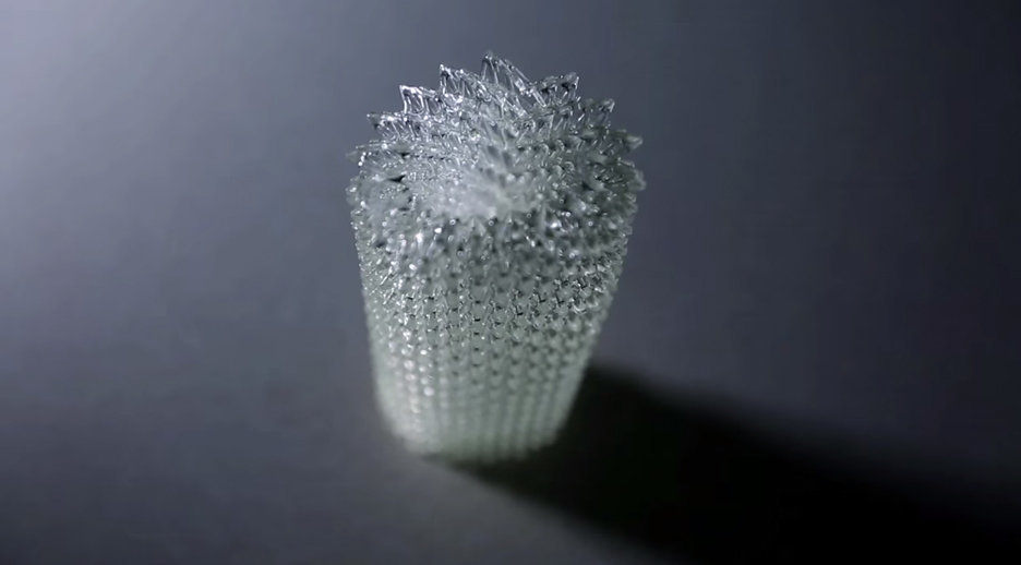
Which means exploding memory cost for things like microstructures

Implicit Representation

Represent geometry as the kernel of a function

Easy to perform boolean operations

Can model essentially arbitrary complexity with low storage overhead

Rendering is time-consuming

You trade space for time

User interaction is not intuitive

Everything is inherently global

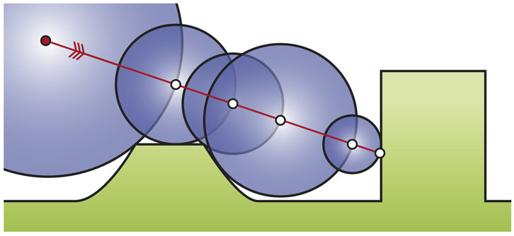
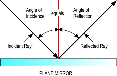
Signed Distance Functions

Special case of implicit representations

The magnitude of the function underestimates the distance to the nearest surface

Underestimation is important because there are some surfaces (looking at you, ellipse) which do not have closed-form distance functions

When (x,y,z) is inside (outside) the surface, the function's sign is positive (negative)

Prior Art

An Example

from math import sqrt
def cylinder(radius):
  def equation(x, y, z):
    return radius - sqrt(x**2 + y**2)
  return equation

my_cylinder = cylinder(1)
assert(my_cylinder(0, 0, 0) == 1) # 1 unit inside cylinder
assert(my_cylinder(1, 0, 0) == 0) # on wall
assert(my_cylinder(2, 0, 0) == -1) # 1 unit outside cylinder

An Example

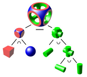
def intersection(f, g):
  def intersected(x, y, z):
    return min(f(x, y, z), g(x, y, z))
  return intersected

def plane(normal, offset):
  def equation(x, y, z):
    a, b, c = normal
    return x*a + y*b + z*c + offset
  return equation

my_plane = plane([0, 0, 1], 0) # as in: this is myPlane get theseSnakes off it!
my_cylinder = cylinder(1)
cut_cylinder = intersection(my_cylinder, my_plane)
assert(cut_cylinder(0, 0, -2) == my_plane(0, 0, -2)) # like a plane below z = 0
assert(cut_cylinder(0, 1, 2) == my_cylinder(0, 1, 2)) # like a cylinder above z = 0

Build Geometry with Closures

Combine primitives lazily

Build a syntax tree in the language of geometries and operations

Rendering Signed Distance Functions

Solving a bunch of equations

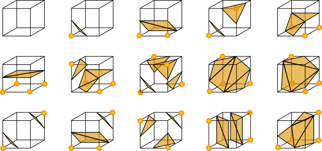
Polygonization

Populate a grid with values of the function and use that grid to approximate the surface with triangles

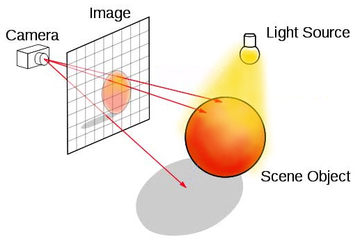
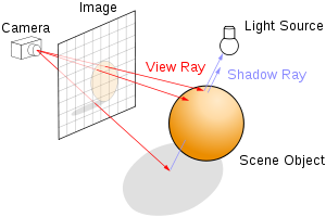
Raytracing

Setup a camera in space, and for each pixel, send a ray to intersect the surface. Draw the intersected points to the screen

Polygonization

Marching Cubes

Raytracing

How can Tensorflow help?

Our representations are trees, and therefore graphs

We would like to:

• Reuse computation results automatically
• Perform efficient computations on large tensors 
• Parallelize!

Tensorflow comes with:

• Common subexpression elimination
• Automatic differentiation
• Compilation to GPU code

Easy to implement*

import tensorflow as tf

cylinder_tf = my_cylinder(tf.constant(0.0), tf.constant(1.0), tf.constant(2.0))
session = tf.Session()
cylinder_tf_result = session.run(cylinder_tf)
assert(cylinder_tf_result == my_cylinder(0, 1, 2))

*Some Tensorflow-specific functions are needed like tf.maximum instead of max

Works with tf.Variable and tf.Placeholder too!

Polygonizing SDFs in Tensorflow

Input a tensor for each coordinate

min_bounds = [-1,-1,-1] # the geometric coordinate bounds
max_bounds = [1,1,1] 
output_shape = [200,200,200]
resolutions = list(map(lambda x: x*1j, output_shape))
mi0, mi1, mi2 = min_bounds
ma0, ma1, ma2 = max_bounds
r0, r1, r2 = resolutions
space_grid = np.mgrid[mi0:ma0:r0,mi1:ma1:r1,mi2:ma2:r2]
space_grid = space_grid.astype(np.float32)
x = tf.Variable(space_grid[0,:,:,:], trainable=False, name="X-Coordinates")
y = tf.Variable(space_grid[1,:,:,:], trainable=False, name="Y-Coordinates")
z = tf.Variable(space_grid[2,:,:,:], trainable=False, name="Z-Coordinates")

draw_op = function(x,y,z)
session = tf.Session()
session.run(tf.initialize_all_variables())
volumetric_grid = tf.session.run(draw_op)
marching_cubes(volumetric_grid) # => list of faces and vertices for rendering

Tensorboard!

Raytracing SDFs in Tensorflow

Solve the equations for t:

First build image plane

def vector_fill(shape, vector):
  return tf.pack([
    tf.fill(shape, vector[0]),
    tf.fill(shape, vector[1]),
    tf.fill(shape, vector[2]),
  ])

resolution = (1920, 1080)
aspect_ratio = resolution[0]/resolution[1]
min_bounds, max_bounds = (-aspect_ratio, -1), (aspect_ratio, 1)
resolutions = list(map(lambda x: x*1j, resolution))
image_plane_coords = np.mgrid[min_bounds[0]:max_bounds[0]:resolutions[0],min_bounds[1]:max_bounds[1]:resolutions[1]]

# Find the center of the image plane
camera_position = tf.constant([-2, 0, 0])
lookAt = (0, 0, 0)
camera = camera_position - np.array(lookAt)
camera_direction = normalize_vector(camera)
focal_length = 1
eye = camera + focal_length * camera_direction

# Coerce into correct shape
image_plane_center = vector_fill(resolution, camera_position)

# Convert u,v parameters to x,y,z coordinates for the image plane
v_unit = [0, 0, -1]
u_unit = tf.cross(camera_direction, v_unit)
uc, vc = image_plane_coords
center = image_plane_center
image_plane = center + uc * vector_fill(resolution, u_unit) + vc * vector_fill(resolution, v_unit)

First build image plane

def vector_fill(shape, vector):
  return tf.pack([
    tf.fill(shape, vector[0]),
    tf.fill(shape, vector[1]),
    tf.fill(shape, vector[2]),
  ])

resolution = (1920, 1080)
aspect_ratio = resolution[0]/resolution[1]
min_bounds, max_bounds = (-aspect_ratio, -1), (aspect_ratio, 1)
resolutions = list(map(lambda x: x*1j, resolution))
image_plane_coords = np.mgrid[min_bounds[0]:max_bounds[0]:resolutions[0],min_bounds[1]:max_bounds[1]:resolutions[1]]

# Find the center of the image plane
camera_position = tf.constant([-2, 0, 0])
lookAt = (0, 0, 0)
camera = camera_position - np.array(lookAt)
camera_direction = normalize_vector(camera)
focal_length = 1
eye = camera + focal_length * camera_direction

# Coerce into correct shape
image_plane_center = vector_fill(resolution, camera_position)

# Convert u,v parameters to x,y,z coordinates for the image plane
v_unit = [0, 0, -1]
u_unit = tf.cross(camera_direction, v_unit)
uc, vc = image_plane_coords
center = image_plane_center
image_plane = center + uc * vector_fill(resolution, u_unit) + vc * vector_fill(resolution, v_unit)

Then build rays

# Populate the image plane with initial unit ray vectors
initial_vectors = image_plane - vector_fill(resolution, eye)
ray_vectors = normalize_vector(initial_vectors)

t = tf.Variable(tf.zeros_initializer(resolution, dtype=tf.float32), name="ScalingFactor")
space = (ray_vectors * t) + image_plane

# Name TF ops for better graph visualization
x = tf.squeeze(tf.slice(space, [0,0,0], [1,-1,-1]), squeeze_dims=[0], name="X-Coordinates")
y = tf.squeeze(tf.slice(space, [1,0,0], [1,-1,-1]), squeeze_dims=[0], name="Y-Coordinates")
z = tf.squeeze(tf.slice(space, [2,0,0], [1,-1,-1]), squeeze_dims=[0], name="Z-Coordinates")

evaluated_function = function(x,y,z)

Then build rays

The iteration operation

Made exquisitely simple because we're using SDF's!

epsilon = 0.0001
distance = tf.abs(evaluated_function)
distance_step = t - (tf.sign(evaluated_function) * tf.maximum(distance, epsilon))
ray_step = t.assign(distance_step)

Just run ray_step as many times as necessary to get convergence

Use automatic differentiation to calculate surface normals for shading

Since the function's value increases as you get closer to the surface, it's derivative always points inward.

Code elided, but here's pictures!

Convert to image

# Mask out pixels not on the surface
epsilon = 0.0001
bitmask = tf.less_equal(distance, epsilon)
masked = color_modulated_by_light * tf.to_float(bitmask)
sky_color = [70, 130, 180]
background = vector_fill(resolution, sky_color) * tf.to_float(tf.logical_not(bitmask))
image_data = tf.cast(masked + background, tf.uint8)

image = tf.transpose(image_data)
render = tf.image.encode_jpeg(image)

Running the iteration

session = tf.Session()
session.run(tf.initialize_all_variables())
step = 0
while step < 50:
  session.run(ray_step)
  step += 1

session.run(render) # <= returns jpeg data you can write to disk

Result in GIF form

Each frame a parameter in the model changes

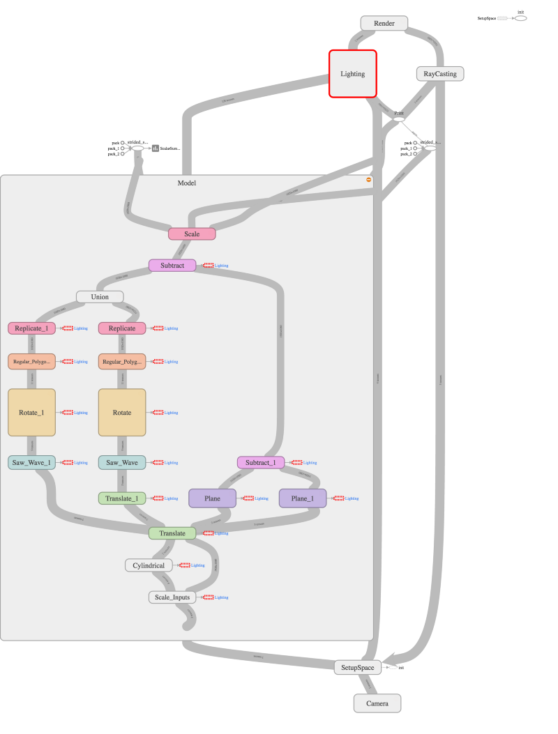
Tensorboard!

Topology Optimization

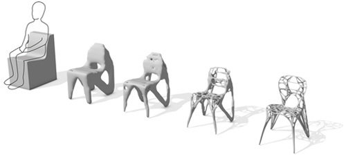
Use tf.Variables in creating the representation and use optimization routines to increase strength to weight ratio

If you want to train on synthetic images, consider rendering them in Tensorflow

That way you have the image data in a tensor and you can calculate per-pixel gradients

Tensorflow is a powerful, generic graph computation framework

With a day job as a neural network library